Fluid Models and Solutions for Large-Scale IP Networks Yong Liu
Francesco Lo Presti
Vishal Misra
Computer Science Department University of Massachusetts Amherst, MA, 01003
Universita’ dell’Aquila Dipartimento di Informatica Via Vetoio (Coppito 1) 67010 Coppito (AQ), Italy
Computer Science Department Columbia University New York, NY 10027
[email protected]
[email protected] [email protected] Don Towsley Yu Gu
Computer Science Department University of Massachusetts Amherst, MA, 01003
Computer Science Department University of Massachusetts Amherst, MA, 01003
[email protected]
[email protected]
ABSTRACT In this paper we present a scalable model of a network of Active Queue Management (AQM) routers serving a large population of TCP flows. We present efficient solution techniques that allow one to obtain the transient behavior of the average queue lengths, packet loss probabilities, and average end-to-end latencies. We model different versions of TCP as well as different versions of RED, the most popular AQM scheme currently in use. Comparisons between our models and ns simulation show our models to be quite accurate while at the same time requiring substantially less time to solve, especially when workloads and bandwidths are high.
Categories and Subject Descriptors C.2 [Computer-Communication Networks]: Miscellaneous ; C.4 [Performance of Systems]: Modeling techniques
General Terms Performance
Keywords Fluid model, Simulation, Large-scale IP networks
1.
INTRODUCTION
Networks, and the Internet in particular, have seen an exponential growth over the past several years. The growth is likely to continue for the foreseeable future, and understanding the behavior of this large system is of critical importance. A problem, however, is that the capabilities of simulators fell behind the size of the Internet a few years ago. The gap has since widened, and is growing almost
Permission to make digital or hard copies of all or part of this work for personal or classroom use is granted without fee provided that copies are not made or distributed for profit or commercial advantage and that copies bear this notice and the full citation on the first page. To copy otherwise, to republish, to post on servers or to redistribute to lists, requires prior specific permission and/or a fee. SIGMETRICS’03, June 10–14, 2003, San Diego, California, USA. Copyright 2003 ACM 1-58113-664-1/03/0006 ...$5.00.
at the same rate as the network is growing. Attempts to close this gap have led to interesting research in the simulation community [5, 2, 3], but we are still someway off in simulating a reasonable sized network. In this paper, we take recourse to scalable modelling as a tool to speed up ”simulations”. Our idea is to abstract out behavior of IP networks into analytical models. Solving the models numerically then yields performance metrics that are close to that of the original networks, thereby enabling an understanding of the key aspects of the performance of the networks. Our starting point is the model in [16] that describes the behavior of TCP networks by a set of (coupled) ordinary differential equations. The differential equations represent the expected or mean behavior of the system. Interestingly, recent results [7, 18] indicate that with appropriate scaling the differential equations in fact represent the sample path behavior, rather than the expected behavior. Hence, our solutions gain in accuracy as the size of the network is increased, a somewhat surprising result. We solve the differential equations numerically, using the Runge-Kutta method, and our simulations show speedups of orders of magnitude compared to packet level discrete event simulators such as ns [4]. Additionally, the time-stepped nature of our solution mode lends itself to a particularly simple parallelization. We also perform a number of optimizations in identifying links that are not bottlenecks to speedup the simulations. The contribution of this paper goes beyond a numerical implementation of the ideas in [16]. We address a number of critical deficiencies of the model in [16]. Most importantly, we incorporate topological information in the set of differential equations. The original model in [16] defined a traffic matrix, which described the set of routers through which a particular set of flows traversed. However, the order in which the flows traversed the routers was absent in the traffic matrix, and that information is potentially of critical importance. In Section 2.2 we exemplify this with a pathological case wherein the model of [16] yields misleading results which our refined model corrects. We also model the behavior of a number of variants of TCP such as SACK, Reno and New-Reno in our model. Going beyond the RED [11] AQM mechanism modelled in [16], we also incorporate other modern AQM mechanisms such as AVQ [15] and PI control [13]. In terms of related work, two works are particularly relevant. In [8], the authors develop fixed point solutions to networks similar
to ones that we are analyzing, to obtain mean performance metrics. However, that approach suffers from two deficiencies. First, we are often interested in transient behavior of the network, that might reveal potential instabilities. Secondly, it is not clear from the solution technique outlined in [8], that the solution complexity scales with the size of the network. Another related approach is that of [17]. In that approach, the authors exploit the model in [16] and the ideas of [7, 18] to demonstrate the fact that the behavior of the network is invariant if the flow population and the link capacities are scaled together. Their approach to simulating large populations of flows in high capacity links is to scale down the system to a smaller number of flows in smaller capacity links, thereby making the simulation tractable for discrete event simulators. The idea is appealing (and in fact applies to our approach too), however the scaling the technique manages is in the population and capacity of the links. Our methodology enables exploring a wider dynamic range of parameters. The time stepped solution technique also lends itself to fairly straightforward parallelization, and we can solve for larger networks (links and routers) than with discrete event simulators. Preliminary results indicate that our computational complexity grows linearly with the size of the network, whereas the growth of the complexity for discrete event simulators is super-linear, providing another win for the fluid based approach. We start with deriving the topology aware fluid model of IP network. Numerical solution algorithm of the fluid model is presented in Section 3. Model refinements are described in Section 4 to account for different versions of TCP and RED implementations. We present some experiment results in Section 5 to demonstrate the accuracy and computation efficiency of our fluid model. Section 6 introduce some extensions to the model. Section 7 concludes the paper and points our directions for future works.
2.
FLUID MODELS OF IP NETWORKS
In this section we present a fluid model for a network of routers serving a population of TCP flows. We will focus on persistent TCP connections working in congestion avoidance stage. Shortlived TCP flows and time-outs are modelled in Section 6.
2.1 Network Model We model the network as a directed graph G = (V, E) where V is a set of routers and E is a set of links. Each link l ∈ E is served at a rate of Cl bps. In addition, associated with each link is an AQM policy, characterized by a probability discarding/marking function pl (t), which may depend on link state such as queue length. Examples, including RED, will be given in Section 2.4. The queue length of l is ql (t), t ≥ 0. Traffic departing from the queue associated with l arrives at the next queue after al seconds. The network G serves a population of N classes of TCP flows. We denote by ni the number of flows in class i, i = 1, . . . , N . The TCP flows within the same class have the same characteristics, follow the same route and experience the same round trip propagation delays. Let Fi = (ki,1 , . . . , ki,m!i ) and Ri = (ji,n! +1 , . . . , ji,mi ) be the ordered set of queues (i.e., links) traversed by the data (forward path) and acks (reverse path) of class i flows, respectively. We distinguish between forward and reverse path as ack traffic (loss) is typically negligible compared to data traffic (loss). Let Ei = Fi ∪ Ri . For k ∈ Ei , we let si (k) and bi (k) denote the queues that follow and precede k, respectively.
2.2 The MGT00 Model In [16], a dynamic model of TCP behavior was developed using a fluid-flow and stochastic differential equation analysis. This model relates the expected values of key TCP flows and network
variables and is described by the following coupled sets of nonlinear differential equations. 1. Windows Size. All flows in the same class will have the same average behavior. Let Wi (t) denote the expected window size of a class i flow at time t. Wi (t) satisfies dWi (t) dt Wi (t) = − λi (t), dt Ri (t) 2 where Ri (t) is the round trip time and λi (t) is the loss indication rate experienced by a class i flow. We defer the expressions for these latter quantities to the next Section. Let Ai (t) denote the (expected) sending rate of a class i flow. This is related to TCP window size by Ai (t) = Wi (t)/Ri (t). 2. Queue Length For each queue l, denote Nl the set of TCP classes traversing queue l. Then: dql (t) = −1(ql (t) > 0)Cl + ni Ai (t), dt i∈N
(1)
l
where 1(expr) stands for the indicator function which assumes value 1 if expr is true, and 0 otherwise. The first differential equation describes the TCP window control dynamic. Roughly speaking, the 1/Ri term models the window’s additive increase , while the Wi /2 term models the window’s multiplicative decrease in response to packet losses, which is assumed to be described by a Poisson process with rate λi (t). The second equation models the queue length behavior as simply the accumulated difference between packet arrival rate at the queue, which in [16] is approximated by term i∈Nl ni Ai (t), and the link capacity Cl . Observe that the approximation arises in replacing the aggregate arrival rate at the queue at time t with the aggregate sending rate of the TCP flows traversing that queue at t. These two quantities can significantly differ for two reasons: (1) flows are shaped as they traverse bottleneck queues; and (2) the arrival rate at time t at a queue is a function of the sending rate at a time t − d, where d is the sum of the propagation and queueing delays from the sender up to the queue. This delay varies from queue to queue and from flow class to flow class. One extreme example is that there is only one TCP class which traverses two identical RED queues with bandwidth C in tandem. The TCP traffic will be shaped at the first queue such that its peak arrival at the second is less than or equal to C, which equals to the service rate at the second queue. Clearly, there won’t be any congestion in the second queue. However, from (1), we will get identical equations for those two queues. Therefore the model predicts the same queue length and packet marking probability for them as shown in Figure 1
2.3
A Topology Aware Model
We have observed in the previous subsection the importance of accounting for the order in which a TCP flow traverses the links on its path. In this section we present a model that takes into account how flows are shaped and delayed as they traverse the network. This is achieved by explicitly characterizing for each class the arrival and departure rate at each queue. For each queue l ∈ Fi traversed by class i flows, let Ali (t) and Dil (t) be the arrival rate and departure rate of a class i flow, respectively. The following sets of expressions relate the departure and arrival process at a queue along the forward path. • Departure Rate When queue length is zero, the departure rate at time t equals the arrival rate. When the queue is not empty,
450
450
ns MGT FFM
400
350
400
300
Queue Length
Queue Length
300
250
200
150
250
200
150
100
100
50
50
0
−50
ns MGT FFM
350
0
0
10
20
30
40
50
60
70
80
90
100
−50
0
10
20
30
40
Time
50
60
70
80
90
100
Time
(a) The First Queue
(b) The Second Queue Figure 1: Importance of Topology Order
the service capacity is divided among the competing flows in proportion to their arrival rates. Thus, for each flow of class i and l ∈ Fi , we have Ali (t), Dil (t)
=
ql (t) = 0
Ali (t−d) Cl , l j∈N Aj (t−d)
(2) ql (t) > 0
l
where d is the queueing delay experienced by the traffic departing from l at time t. d can be obtained as the solution of the following equation ql (t − d) = d. Cl
Ai (t), =
b (l)
Di i
To compute λi (t) we need to consider the fate of the unit of traffic that departs at time t − Ri (t) at each node along the forward path (assuming ack loss is negligible). Thus, Ali (tl )pl (tl )
λi (t) =
(8)
l∈Fi
2. Queue Length
l = ki,1 (4)
(t − abi (l) ),
where tki,1 = t.
(3)
• Arrival Rate For each flow of class i, its arrival rate at the first queue on its route is just its sending rate. On any other queue, its arrival rate is its departure rate from its upstream queue after a time lag of link propagation delay. It is summarized in the following equation: Ali (t)
where tl is the time at which the data or ack arrived at queue l. {tl , l ∈ Ei } are related to t by the following set of equations: ql (tl ) tsi (l) = al + tl + (7) Cl
otherwise
The system evolution is governed by a set of differential equations: 1. Window Size.
For each queue l, denote Nl the set of TCP classes traversing it. Then: dql (t) ni Ali (t) (9) = −1(ql (t) > 0)Cl + dt i∈N l
We repeat the tandem queue experiment in Section 2.2. Revised topology order aware model gives accurate queue length results at both queues as shown in Figure 1
2.4 AQM Policies The classical example of an AQM policy is RED [11]. The differential equation governing pl (t) is described by the following: RED computes the marking probability based upon an average queue length x(t). The relationship is defined by the following:
The window size Wi (t) of a flow of class i satisfies 1(Wi (t) < Mi ) Wi (t) dWi (t) = − λi (t) dt Ri (t) 2
(5)
where Mi is the maximal TCP window size, Ri (t) and λi (t) denotes the round trip time and the loss indication rate at time t (in other words, as seen by the sender at time t). Ri (t) is such that t − Ri (t) is the time at which the data, whose ack has been received at time t, departed the sender. Ri (t) takes the form Ri (t) = l∈Fi ∪Ri
ql (tl ) al + Cl
(6)
0, min
x−t p tmax −tmin
p(x) =
max
1,
0 ≤ x < tmin , tmin ≤ x ≤ tmax tmax < x
(10)
where tmin , tmax , and pmax are configurable parameters. In the gentle variant of RED, the following modification is done: 0, p(x) =
x−tmin pmax , tmax −tmin x−tmax (1 − pmax ) tmax
0 ≤ x < tmin tmin ≤ x ≤ tmax max +p , tmax < x ≤ 2tmax (11)
In [16], the differential describing x(t) was derived to be dx loge (1 − α) loge (1 − α) = x(t) − q(t) (12) dt δ δ where δ and α are the sampling interval and the weight used in the EWMA computation of the average queue length x(t). Thus, the differential equation describing pl (t) is obtained by appropriately scaling (12) with (10) or (11) according to the scheme used. Another AQM scheme PI [13] has the following differential equation describing pl (t): The PI controller tries to regulate the error signal e(t) between the queue length q(t) some desired queue length qref (e(t) = q(t) − qref ). In steady state the PI controller drives the error signal to 0. The relationship between pl (t) and q(t) is described by dpl dq(t) = K1 + K2 (q(t) − qref ) (13) dt dt where K1 and K2 are design parameters of the PI algorithm. Note that the REM algorithm uses a similar differential equation to compute the price at a link, which is subsequently used by a static function to compute the marking probability. Thus, the same scheme as PI works with a little modification for REM. We have a similar description for AVQ but due to space constraints we have not included it in this paper.
2.5 Model Reduction In most operating networks, congestion only occurs in several spots, such as access points and peering points of ISPs. Most network links, especially in backbone networks, operate at low utilization level. Queues at those links will be always empty and no packet will be dropped there. Therefore there is no need to model queueing and RED behavior and maintain TCP states on those links. The network model can be reduced so that we only solve queueing and RED equations for potentially congested links and those uncongested links are transparent to all TCP classes except for introducing propagation delays. It will greatly reduce the computation time of the fluid model solver. Given a network topology and traffic matrix, we can identify uncongested links as follows:
queue on its route is bounded by the ratio of its maximal congestion window to its two way propagation delay.
3. TIME-STEPPED MODEL SOLUTION ALGORITHM The solution of the fluid model can be obtained by solving the group of delayed differential equations defined in (2)-(13) at a low computational cost. We have implemented our fluid model solution in both Matlab and C. Matlab has its own Ordinary Differential Equation (ODE) solver suite. As a script language, Matlab is far from being optimized in terms of computation cost and doesn’t provide much programming flexibility. Alternatively, we programmed fixed step-size Runge-Kutta algorithm [9] in C to solve the fluid model. The Runge-Kutta algorithm is a widely used method to solve differential equations numerically. Briefly, for a system described by dy(t) = f (t, y(t)), dt where y(t) = {y1 (t), y2 (t), · · · , ym (t)}, its solution can be obtained by the numerical integration y((n + 1)h) = y(nh) +
h [kn,1 + 2kn,2 + 2kn,3 + kn,4 ], 6
where h is the solution step-size and kn,1 kn,2 kn,3 kn,4
= f (tn , y(nh)) = f (tn + h/2, y(nh) + kn,1 h/2) = f (tn + h/2, y(nh) + kn,2 h/2) = f (tn + h, y(nh) + kn,3 h)
By implementing the Runge-Kutta algorithm, the fluid model solver essentially becomes a time-stepped network simulator. Figure 2 depicts the flowchart of fluid model solver. After reading in network topology and TCP traffic matrix from a configuration file, the fluid model solver conducts model reduction using the algo• Step 1 Define queue adjacent matrix ADJ such that ADJ(i, j) = rithm in Section 2.5. Then the fluid model is solved step by step for the whole duration of simulated time. At each time step, the send1 if there exists a TCP class which traverses queue j immeing rate of each TCP class is updated according to (5); queue length diately after it traverses queue i; ADJ(i, j) = 0 otherwise. and packet loss probability at each congested queue are calculated For queue i, define set O(i) as the set of TCP classes which from (9) and corresponding AQM equations, e.g. (10,11 and 12) have queue i as their first hop. for RED; TCP state variables {Ri (t), λi (t), Ali (t), Dil (t)} are up• Step 2 Queue i is marked as uncongested if dated according to equations (2,4,6,8). The solution of the fluid model, including the sending rate of each TCP class and each conMk nk < Ci , (14) ADJ(l, i) ∗ Cl + gested queue’s packet loss probability and queue length, is dumped pdk l∈E into data files at the end of the process. k∈O(i) To solve equations (2,4,6,8) directly, for each t, we would need where Mk is the maximal TCP window size, nk is the flow to track back in time for each class the instant at which data (ack) population and pdk is two way propagation delay of TCP arrived at each queue. Instead, we find it convenient to proceed by class k. rewriting those equations forward in time, i.e., by expressing the future value of the round trip time, loss rate indication, arrival and • Step 3 Remove all uncongested queues from the topology departure rate as function of their current values. We proceed as and adjust TCP route accordingly. If all queues on a TCP follows: class’s route have been removed, remove this TCP class and calculate its sending rate as Mk nk /pdk . • Round Trip Time • Step 4 If no queue is removed in Step 3, end the model Let dil (t), l ∈ Ei , i = 1, . . . , N , be the total delay accrued reduction; otherwise, go back to Step 1. by the unit of data (ack) which at time t has arrived to node l. From the definition, The first term on left hand side of (14) is the queue i’s maximal traffic inflow rate from all its upstream queues. The second term Ri (t) = disi (t) (15) accounts for the fact that a TCP flow’s arrival rate at the very first
The accuracy of the solution of a differential equation system is determined by the stiffness of the system and the solution step-size. The smaller the step-size the more accurate the solution. On the other hand, the computation cost of our time-stepped fluid model solver is proportional to its step-size. For our fluid model solver, the tradeoff between step-size and solution accuracy is not stringent. The stiffness of the fluid network model is bounded by the smallest round trip time of TCP classes and the highest bandwidth of congested queues. We can achieve accurate enough results with a small enough step-size. Meanwhile our fluid model solver still runs fast even with a small step-size. As we will see in Section 5, a step-size of 1ms is small enough for our fluid model solver to get accurate solution and at the same time enables the solution of a large IP network to be obtained reasonably fast.
Start
Initialiazation
End of Simulation?
NO Update Windows of All TCP Classes
Update Queue Length & Loss Probability at all Congested Link
YES
4. REFINEMENTS OF FLUID MODEL Model in Section 2 captures the basic dynamic behavior of TCP and RED. Implementation details change their behavior to certain extent. In this section, we present some model refinements which account for a variety of detailed behavior of both TCP and RED.
Update Each TCP State Variables at All Queues on its Route
4.1 Variants of TCP Dumping Data
END
Figure 2: Flowchart of Fluid Model Solver We compute these delays forward in time as follows: qbi (l) (t) + abi (l) , Cbi (l)
dil (tf ) = dibi (l) (t) + where tf = t +
qb (l) (t) i Cb (l) i
(16)
+ abi (l) is the data arrival time at
link l given that those data arrive at its previous link bi (l) at time t. • Loss Rate Indication
Let rli (t), l ∈ Ei , i = 1, . . . , N , be the amount out of the data arriving at link l at time t which was lost. From the definition, we have λi (t) = rsi i (t) rli (tf )
=
(17)
rbi i (l) (t)
+
b (l) Ai i (t)pbi (l) (t)
l ∈ Fi
rli (tf ) = rbi i (l) (t)
l ∈ Ri
(18) (19)
• Departure Rate
The expressions for the departure rate are directly obtained from (2). For each class i and l ∈ Fi Dil t +
ql (t) Cl
=
Ali (t) Ali (t) Cl l j∈N Aj (t)
ql (t) = 0 ql (t) > 0
(20)
l
• Arrival Rate
For each flow i and l ∈ Fi , b (l)
Ali (t + abi (l) ) = Di i
(t)
(21)
Equation (5) models the behavior of TCP Reno. Starting from the Reno version, TCP implements Fast Recovery mechanism. TCP halves its congestion window whenever the number of duplicated ACKs crosses a threshold. When there are multiple packet losses in a window, TCP Reno reduces its window several times. This makes Fast Recovery inefficient. New Fast Recovery mechanisms are implemented in Newreno and SACK to ensure at most one window reduction for packet losses within one window. In [10], simulation results show Newreno and SACK recover much faster than Reno from multiple packet losses. To model the Fast Recovery mechanisms of Newreno and SACK, we replace perceived packet loss rate λi (t) in Equation (5) by Effective Loss Rate λ$i (t) =
1 − (1 −
λi (t) )Ri (t)Ai (t−Ri (t)) Ai (t−Ri (t))
Ri (t)
λi (t)/Ai (t−Ri (t)) approximates the end-to-end packet loss probability. Consequently, the numerator is the probability of at least one packet is lost within a window of Ri (t)Ai (t − Ri (t)) packets. Therefore λ$i (t) models the actual window back off rate for TCP Newreno and SACK under loss indication rate λi (t). When the packet loss probability λi (t)/Ai (t − Ri (t)) is small, we will have λ$i (t) ≈ λi (t).
4.2 Compensation for Variance of TCP Windows From equation (5), in stationary state, we will have W = 2/p. Other studies [6, 14] predict W = 1.5/p. We think the difference comes from the assumption on loss event process. Our model is a mean-value model: we model only the first order statistics of TCP window sizes and queue lengths. In a real network, those second order statistics, e.g. variance of TCP window size, impact on network stationary behavior. For example, we use average window size to approximate TCP’s window size before back off. This is accurate if loss arrival is independent of TCP window. When the correlation between a TCP class’s window size and perceived loss arrival is not negligible, some compensation is necessary. One extreme example is a single bottle-neck supporting a single TCP class of M flows. Let W i denote the window size of ith flow within this M i ¯ = 1 class. The average window size of the class is W i=1 W . M
Given a small packet loss probability p, the probability that at least one packet in a window will be dropped is approximately W i p. Then the average back off for the whole class is 1 M
M
(W i )2 p/2,
S1
Class 2
S2
Class 3
S3
D1
B1
B2
D2
i=1
¯ 2 p/2. To demonstrate, we conduct an which will be bigger than W ns simulation of a single bottle-neck serving single-class of TCP flows and measure each TCP flow’s window size immediately before back off. From Figure 3 TCP window sizes before back-offs is generally bigger than the average window size . To compensate,
D3
Figure 6: Single bottle-neck network with dynamic workload probability 1 if count × p ≥ 2. Inter-marking interval X is uniformly distributed in [1/p, 2/p]. It effectively reduces the packet marking probability 2p/3.
45
Average Mean Window Size
40
Class 1
35
To account for those implementation details, we change the calculation of the RED marking probability in the fluid model as
30
25
pl (t) =
20
15
10
5
0 20
30
40
50
60
70
80
90
100
Time
Figure 3: TCP Window Sizes prior to Back-offs ¯ /1.5 instead of W ¯ /2 to model average back off of a TCP we use W flow. Figure 4 contains results for ns and fluid model with Multiplicative Decrease factor M D = 1.5 and M D = 2.
4.3 RED Implementation Adjustments In this section, we model different versions of RED implementation. • Geometric and Uniform After calculating the packet marking probability p based on average queue length, RED marks packet independently with p. Let X be the time interval between two marks. Then X assumes a geometric distribution P (X = k) = (1 − p)k−1 p In [11], authors point out that a geometric inter-marking time will cause global synchronization among connections. They then propose a marking mechanism to make X uniformly distributed in [1, 1/p]. Each arriving packet is marked with probability p/(1 − count × p), where count is the number of unmarked packets that have arrived since the last marked packet. A packet will always be marked if count × p ≥ 1. By doing this, the actual packet marking probability is approximately 2p. To account for uniform dropping, packet marking probability of RED is calculated in fluid model as pl (t) = 2 ∗ p(xl (t)), where p(·) is the piece wise linear RED marking profile as defined in (11). • Wait Option In the ns implementation, a RED option wait is introduced to avoid marking two packets in a row. When wait option is on, which is default for a recent ns version, an arriving packet is marked with probability p/(2 − count × p) if 1 ≤ count × p ≤ 2. A packet will be marked with
2 p(xl (t)) 3
2p(xl (t))
wait = 1 wait = 0
We did a simulation on a single bottle-neck network with a single TCP class of 60 flows. The RED queue at the bottle-neck uses ECN marking. Figure 5 shows the results for the RED queue with and without wait option. Notice that the packet marking probability predicted by our fluid model is a little higher than the actual packet marking rate in ns. This is because we don’t model Timeout and will need a higher packet marking rate to bring down the TCP sending rates.
5. EXPERIMENTAL RESULTS We have performed extensive experiments to evaluate the accuracy and computation efficiency of our fluid models. Given the limited space, we are only able to present several representative experiments here. More results are available for interested readers. For all experiments in this section, we use TCP Newreno and RED with ECN marking as AQM policy. Stepsize of fluid model solver is fixed at 1ms. We start with a single bottle-neck topology with a variable TCP workload. The fluid model’s accuracy is tested by comparing its solution with simulation results obtained in ns when the network operates in both stable and unstable regions. In Section 5.2, the fluid model’s scalability is demonstrated on a two bottleneck topology. The results show that the fluid model is scalable in the link bandwidth and flow populations. In addition, its accuracy improves as the link bandwidth scales up. In the last experiment, we test the capacity of our fluid model based simulation on a large topology with more than 1, 000 nodes and thousands of TCP classes consisting up to 176, 000 TCP flows. Computation results show that the fluid model approach is promising in simulating large IP networks.
5.1 Accuracy of Fluid Model The first experiment is to demonstrate the accuracy of our fluid model. As shown in Figure 6, there are 3 TCP classes sharing a bottle-neck link with bandwidth of 10M bps. Each TCP class consists of 20 homogeneous TCP flows. There are totally 14 queues. After model reduction, fluid model only need to simulate 4 queues which potentially have congestion. TCP class 1 and 2 start at time 0. After 40 seconds, class 2 stop sending data. The number of TCP flows on the bottle-neck link reduced from 40 to 20. The system enters unstable region. At 70 second, both class 2 and class 3 become active. TCP workload increases by a factor of 3. The system
22
0.03
20
MD=2 MD=3/2 NS
MD=2 MD=3/2 NS
0.025
Packet Marking Prob.
Average Window Size
18 16 14 12 10 8 6 4
0.02
0.015
0.01
0.005
2 0 20
25
30
35
40
45
0 20
50
25
30
35
Time
40
45
50
Time
(a) Window Size
(b) Loss Probability Figure 4: Compensation for Window Variance
160
120
NS FFM w/o Adj. FFM w. Adj
100
NS FFM w/o Adj. FFM w. Adj
120
Average Queue Length
Average Queue Length
140
100
80
60
40
80
60
40
20 20
0
0 5
10
15
20
25
30
35
40
5
10
15
20
Time
Time
(a) wait is on
(b) wait is off Figure 5: Account for RED Implementations
25
30
35
40
80
500
450
NS Sample NS Average FFM
60
400
NS FFM
350
Queue Length
Window Size (Group1)
70
50
40
30
300
250
200
150 20 100 10
0
50
20
30
40
50
60
70
80
90
100
0
20
30
40
50
Time
60
70
80
90
100
Time
(a) TCP Window Size
(b) Bottle-neck Queue
Figure 7: Results for Single Bottleneck Topology
3 Class3 1
5 Class1
2
4
6
8 Class2
7
K ns FFM Speedup
1 12.5 0.766 16.32
10 122 0.766 159.3
50 983 0.766 1,283
100 1,676 0.766 2,188
Table 1: Computation Cost of ns and Fluid Model
9
Figure 8: Network with Two Bottlenecks eventually settles around its stable operation point. We compare the fluid model solution with results obtained from ns. Figure 7(a) plots one TCP connection’s window sample path and the average window size we obtained from both ns and fluid model. The fluid model captures the average window behavior very well both when the system is stable and unstable. Figure 7(b) plots instantaneous queue length from ns and the average queue length predicted by the fluid model. We also see a good match, which also implies the fluid model calculates RED packet marking probability accurately.
5.2 Model Scalability with Link Bandwidth The second set of experiments is to show fluid model’s scalability with link bandwidth and flow populations. We set up 3 TCP classes on a network of 8 links as in Figure 8. Link bandwidth and flow population within each class are set to be proportional to a scale parameter K, which ranges from 1 to 100. The link between node 2 node 4 and the link between node 6 and 8 have bandwidth of K ∗ 10M bps. Other links have bandwidth of K ∗ 100M bps. Each TCP class consists of K ∗ 40 TCP flows. In order for simulation results at different scales to be comparable, we change RED thresholds tmin and tmax proportional to K and its queue averaging weight α inversely proportional to K. There are totally 16 queues in the network. Our model reduction algorithm identifies 12 of them as uncongested queues which don’t need to be simulated. For each K, we run a simulation of 100 seconds using both ns and fluid model solver. Figure 9 and Figure 10 show simulation results for K = 1 and K = 10 respectively. ns simulation results eventually converge to fluid model solution when K gets bigger. Because the fluid model is scalable with both link bandwidth and flow population, the computation cost to obtain model
solution is invariant to the scale parameter K. On the other hand, packet events in ns grows as link bandwidth and number of flows scale up. It takes much longer for ns simulation to finish when K = 100 than K = 1. Table 1 lists pure computation costs in unit of second of ns and the fluid model, both without dumping data. The larger the scale, the bigger computation savings for the fluid model.
5.3 Experience with Large IP Networks In this experiment, we test the capacity of our fluid model based simulation approach on a large IP network with structured topology. The simulated topology is adapted from a baseline network model [1] posed as a challenge to large network simulators by the DARPA Network Modelling and Simulation program. At a high level, the topology can be visualized as a ring of N nodes. Each node in the ring represents a campus network and is connected to its two neighbors by links with bandwidth of 9.6Gbps and random delay uniformly distributed in the range of 10-20ms. In addition, each node is connected to a randomly chosen node other than its neighbors through a chord link. Figure 11(a) is a ring structure generated for N = 20. The campus networks at all nodes share the same topology shown in Figure 11. Each campus network consists of 4 sub-networks: Net 0, 1, 2, 3. All the links in campus networks have bandwidth of 2.5Gbps. Node 0.0 in Net 0 acts as the border router and connects to border routers of other campus networks. The links within Net 0 have random delays uniformly distributed in the range of 5 − 10ms. Links connecting 0.x to other sub-networks have random delays uniformly distributed in the range of 1 − 5ms. All links in Net 1, Net 2 and Net 3 have random delays of 1-2ms. Net 1 contains two routers and four application servers. Net 2 and Net 3 each contains four routers connecting to client hosts. The traffic contains persistent TCP flows. From each router in
80
250
NS Class1 FFM Class1 NS Class3 FFM Class3
70
200
Queue Length
Sending Rate
60
NS Bottleneck1 FFM Bottleneck1 NS Bottleneck2 FFM Bottleneck2
50
40
30
150
100
20 50 10
0 10
15
20
25
30
35
40
45
0 10
50
15
20
25
Time
30
35
40
45
50
40
45
50
Time
(a) TCP Sending Rate
(b) Bottle-neck Queues Figure 9: Simulation Results when K = 1
80
2500
NS Class1 FFM Class1 NS Class3 FFM Class3
70
Queue Length
Sending Rate
60
NS Bottleneck1 FFM Bottleneck1 NS Bottleneck2 FFM Bottleneck2
2000
50
40
30
1500
1000
20 500 10
0 10
15
20
25
30
35
40
45
50
0 10
15
20
Time
25
30
35
Time
(a) TCP Sending Rate
(b) Bottle-neck Queues
Figure 10: Simulation Results when K = 10
1.2 0.2
1.0 1.3 Net 1
Net 0
1.4 0.0
0.1
1.1 1.5
4
2.0
5
2.1
3.1
Net 3
Net 2
2.2
3.0
2.3
3.2
3.3
(b) Topology of Subnetworks
(a) Ring Structure
Figure 11: Topology of a Large IP Network
approach is promising in simulating large IP networks. Numerical solution gives us plenty of flexibility to extend the fluid model without worrying about the complexity of solving them analytically. In this section, we present some model extensions which we have done but haven’t conducted extensive validations for.
4500 4000 3500
Time (s)
3000 2500 2000
6.1 Model Time-out and Slow Start
1500 1000 500 0
0
10
20
30
40
50
60
N
Figure 12: Computation Cost as a function of N Net 2 and Net 3, there are 8 TCP classes. Four of them are destined at servers in its neighboring campus network. The other four classes are destined at servers in the campus network which connects to it through a chord link. Each TCP class contains K homogeneous TCP flows. In total, the entire network has 19N nodes, 44N queues, and 64N TCP classes. Our experiment is carried on a Dell Precision Workstation 530, which is configured with two Pentium IV processors(2.2GHz) and 2GB memory. However, our program is not parallelized. Therefore only one processor is utilized. We fix the flow population of each TCP class at 50 and vary the number of campus networks on the ring from 5 to 55. Each topology is simulated for 100 seconds. Our model reduction algorithm identifies 59.1% queues as uncongested. Figure 12 illustrates simulation times that grow almost linearly with the number of campus networks. The simulation for the largest topology, which consists of 1, 045 nodes and 176, 000 TCP flows, finished after 74 minutes and 7.2 seconds.
6.
EXTENSIONS AND FUTURE WORKS We have seen in previous sections that our fluid model based
The model described in Section 2 captures the additive increase multiplicative decrease dynamic of the TCP window control. As shown in [16], the model can be easily extended to account for timeout losses and the slow start behavior of TCP, by replacing (5) with Wi (t) dWi (t) 1 = (1 − αi,CA ) + αi,CA dt Ri (t) Ri (t) Wi (t) − λi (t)(1 − pi,T O ) − (Wi (t) − 1)λi (t)pi,T O 2
(22)
The Wi /Ri term models the exponential growth of the window size in the slow start phase of TCP, while the Wi − 1 term models the window’s reduction to 1 in response to timeout losses. αi,CA is the probability that a flow of class i is in congestion avoidance (CA). For long lived flows, we can ignore the slow start phase and set αi,CA = 1. For short lived flow, on the other hand, they are always in slow start, and we can set αi,CA = 0. pi,T O is the probability that a loss is a timeout loss. This probability can be approximated by pi,T O = min{1, 3/Wi } ([14]).
6.2 Incorporate Unresponsive Traffic Although the majority of Internet traffic is controlled by TCP, a non-negligible amount of traffic is unresponsive to congestion. It can be generated by either UDP connections or simply TCP connections which are too short to experience congestion. A recent work [12] studies unresponsive traffic’s impacts on AQM performance based on the MGT model. We can incorporate unresponsive
traffic into our model by changing (9) to dql (t) = −1(ql (t) > 0)Cl + ni Ai (t) + ul (t), dt i∈N
(23)
l
where ul (t) is aggregate unresponsive traffic rate at queue l. Instead of generating individual unresponsive flows, we can use different unresponsive traffic rate models derived in [12] for ul (t) to speed up our simulation.
7.
CONCLUSIONS AND FUTURE WORKS
In this paper, we have developed a methodology to obtain performance metrics of large, high bandwidth IP networks. We started with the basic fluid model developed in [16], and made considerable improvements and enhancements to it. Most importantly, we made the model developed in that paper topology aware. That contribution alone is of independent interest in terms of theoretical (fluid) studies of such networks, as topology awareness can play a critical part in conclusions regarding stability and performance as we demonstrated by a simple tandem queue example. We also incorporated a number of TCP features and variants, as also a number of different AQM schemes into the model. Our solution methodology is computationally extremely efficient, and the scalable model enables us to obtain performance metrics of high bandwidth networks that are well beyond the capabilities of current discrete event simulators. Our technique also scales well with the size of the network, displaying a linear growth in computational complexity, as opposed to a super-linear one observed with discrete event simulators. The time stepped nature of our solution lends itself to a straightforward parallel implementation, pointing to another possible avenue of ”simulating” large networks. As a future work, we will further extend the fluid model and at the same time validate model extensions, including those described in the previous section. Model reduction algorithm described in Section 2.5 still has some space to improve. Another exciting future work direction is to integrate our fluid model based simulator with other existing packet level simulators to conduct hybrid simulation. In such a hybrid simulation, our fluid simulator can be used to simulate back ground traffic in the core network and provide network delay and loss information to packet traffic running across the fluid core. Preliminary attempts to integrate our fluid simulator with ns have proven successful. Now we are working on integrating our fluid simulator with parallel packet level simulators in a distributed fashion to further boost its simulation speed.
8.
REFERENCES
[1] DARPA NMS Baseline Network Topology. http://www.cs.dartmouth.edu/∼nicol/NMS/baseline/. [2] Parallel and Distributed NS. http://www.cc.gatech.edu/computing/compass/pdns/.
[3] Scalable Simulation Framework (SSFNet). http://www.ssfnet.org. [4] The Network Simulator - ns-2. http://www.isi.edu/nsnam/ns/. [5] Virtual InterNetwork Testbed. http://www.isi.edu/nsnam/vint/. [6] E. Altman, K. Avrachenkov, and C. Barakat. A stochastic model of TCP/IP with stationary random losses. In Proceedings of ACM/SIGCOMM ’00, September 2000. [7] F. Baccelli, D. McDonald, and J. Reynier. A Mean-field Model for Multiple TCP Connections through a Buffer. In Proceedings of IFIP WG 7.3 Performance, 2002. [8] T. Bu and D. Towsley. Fixed Point Approximation for TCP behavior in an AQM Network. In Proceedings of ACM/Sigmetrics, 2001. [9] J. W. Daniel and R. E. Moore, editors. Computation and theory in ordinary differential equations. San Francisco, W. H. Freeman, 1970. [10] K. Fall and S. Floyd. Simulation-based comparisons of Tahoe, Reno, and SACK TCP. Computer Communications Review, 26, July 1996. [11] S. Floyd and V. Jacobson. Random Early Detection gateways for congestion avoidance. IEEE/ACM Transactions on Networking, 1(4):397–413, August 1993. [12] C. Hollot, Y. Liu, V. Misra, and D. Towsley. Unresponsive flows and AQM performance. In Proceedings of IEEE/INFOCOM, 2003. [13] C. Hollot, V. Misra, D. Towsley, and W.-B. Gong. On Designing Improved Controllers for AQM Routers Supporting TCP Flows. In Proceedings of IEEE/INFOCOM, April 2001. [14] J.Padhye, V. Firoiu, D. Towsley, and J. Kurose. Modeling tcp throughput: A simple model and its empirical. In Proceedings of ACM/SIGCOMM ’1998, 1998. [15] S. Kunniyur and R. Srikant. Analysis and design of an adaptive virtual queue algorithm for active queue management. In Proceedings of ACM/SIGCOMM ’2001, 2001. [16] V. Misra, W.-B. Gong, and D. Towsley. Fluid-based Analysis of a Network of AQM Routers Supporting TCP Flows with an Application to RED. In Proceedings of ACM/SIGCOMM, 2000. [17] K. Psounis, R. Pan, B. Prabhakar, and D. Wischik. The scaling hypothesis: simplifying the prediction of network performance using scaled-down simulations. ACM Computer Communications Review, January 2003. [18] P. Tinnakornsrisuphap and A. Makowski. Limit Behavior of ECN/RED Gateways Under a Large Number of TCP Flows . In Proceedings of IEEE Infocom, 2003.