fluid-structure interaction boundary conditions by artificial compressibility

European Communityon Computational Methods in Applied Sciences ECCOMAS Computational Fluid Dynamics Conference 2001 Swansea, Wales, UK, 4-7 September 2001 c
ECCOMAS

FLUID-STRUCTURE INTERACTION BOUNDARY CONDITIONS BY ARTIFICIAL COMPRESSIBILITY Peter R˚ aback, Juha Ruokolainen, Mikko Lyly, and Esko J¨ arvinen CSC – Scientific Computing Ltd., Box 405, FIN-02101 Espoo, e-mail: Peter.Raback@csc.fi, web-page: http://www.csc.fi

Key words: Fluid-structure interaction, artificial compressibility, incompressible NaviesStokes, finite element method Abstract. An automated method for solving fluid-structure interaction (FSI) problems is presented. In the method the initially incompressible fluid is given an artificial compressibility that corresponds to the elastic properties of the stucture. The compressibility is continuously updated by using the current pressure field as a test load. The compressibility may be uniform or have a predefined profile. When the coupled iteration converges also the effect of the artifical compressibility vanishes. The method is implemented and successfully applied to 2D and 3D test cases with large deformations.

1

Peter R˚ aback, Juha Ruokolainen, Mikko Lyly, and Esko J¨ arvinen

1

INTRODUCTION

When fluid-structure interaction (FSI) problems are solved with a loosely coupled iteration strategy there is a risk of applying unphysical boundary conditions that lead to severe convergence problems. The reason for this is that initially the fluid domain is unaware of the constraint of the structural domain, and vice versa. If the iteration converges this discrepancy will be settled, but sometimes the initial phase is so ill posed that convergence is practically impossible to obtain. Imagine an elastic container with inlets only. In the start of the iteration the walls are at rest which results to zero velocity boundary conditions. If the fluid is incompressible there is no way to satisfy the continuity equation as there is a net flux into the container. This problem has been clearly demonstrated in the modeling of fluid-structure interaction of human artery. The convergence problems have been found to increase with the length of the artery. Some computations require relaxation factors below 0.01, which seriously limits the computational efficiency [1, 2]. The problem may be approached by applying the method of artificial compressibility to the fluid-structure interaction [3]. Artificial compressibility has been previously used mainly as a trick to eliminate the pressure from the Navies-Stokes equations or to improve the convergence of the solution procedure [4, 5, 6]. In fluid-structure interaction the artificial compressibility follows a different argumentation and has a natural physical explanation: The compressibility is defined so that it makes the fluid imitate the elastic response of the structure. 2

FLUID-STRUCTURE INTERACTION

We look at the time-dependent fluid-structure interaction of elastic structures and incompressible fluid. The equations of momentum in the structural domain is ∂ 2u = ∇ · τ + f in Ωs , (1) ∂t2 where ρ is the density, u is the displacement, f the applied body force and τ = τ (u) the stress tensor that for elastic materials may be locally linearized with u. For the fluid fluid domain the equation is ρ





∂v ρ + v · ∇v = ∇ · σ + f in Ωf , ∂t

(2)

where v the fluid velocity and σ the stress tensor. For Newtonian incompressible fluids the stress is σ = 2µε(v ) − pI, (3) where µ is the viscosity, ε(v ) the strain rate tensor and p the pressure. In addition the fluid has to follow the equation of continuity that for incompressible fluid simplifies to ∇ · v = 0 in Ωf . 2

(4)

Peter R˚ aback, Juha Ruokolainen, Mikko Lyly, and Esko J¨ arvinen

For later use we, however, recall the general form of the continuity equation, ∂ρ + ∇ · (ρv ) = 0 in Ωf . ∂t

(5)

The fluid-structure interface, Γf s , must meet two different boundary conditions. At the interface the fluid and structure velocity should be the same, v (r, t) = u˙ (r, t), r ∈ Γf s .

(6)

On the other hand, the surface force acting on the structure, gs , should be opposite to the force acting on the fluid, gf , thus gs (r, t) = −gf (r, t), r ∈ Γf s .

(7)

A widely used iteration scheme in FSI is the following: First, assume a constant geometry and solve the Navier-Stokes equation for the fluid domain with fixed boundary conditions for the velocity. Then calculate the surface forces acting on the structure. Using these forces solve the structural problem. Using the resulting displacement velocities as fixed boundary conditions resolve the fluid domain. Continue the procedure until the solution has converged. The above described iteration usually works quite well. However, in some cases the boundary conditions (6) and (7) lead to problems. The elasticity solver is not aware of the divergence free constraint of the velocity field. Therefore the suggested displacement velocities used as boundary conditions may well be such that there is no solution for the continuity equation. A proper coupling method makes the solution possible even if the velocity boundary conditions aren’t exactly correct. Further, if the Navier-Stokes equation is solved without taking into account the elasticity of the walls, the forces in equation (7) will be exaggerated. The pathological case is one where all the boundaries have fixed velocities. Then even an infinitely small net flux leads to infinite pressure values. A proper coupling method should therefore also give realistic pressure values even with inaccurate boundary conditions. The method of artificial compressibility meets both these requirements. 3

ARTIFICIAL COMPRESSIBILITY

When a surface load is applied to an elastic container it results to a change in the volume. In many cases of practical interest the change in volume is mainly due to a pressure variation from the equilibrium pressure that leads to zero displacements. If the structural domain is described by linear equations the change in volume dV has a direct dependence on the change in the pressure, dP , or dV = c dP. V 3

(8)

Peter R˚ aback, Juha Ruokolainen, Mikko Lyly, and Esko J¨ arvinen

This assumption limits the use of the model in highly nonlinear cases. The change in the volume should be the same as the net volume flux into the domain. As this cannot be guaranteed during the iteration, some other way to enable the material conservation must be used. A natural choice is to let the density of the fluid vary so that is has the same pressure response as the elastic walls, dρ = c dP, ρ

(9)

where c is the artificial compressibility. This is interpreted locally and inserted to the continuity equation (5) while neglecting the space derivative of the density, thus c

dp + ∇ · v = 0, dt

(10)

where dp is the local pressure change. Here the time derivative of pressure must be understood as an iteration trick. A more precise expression is  c  (m) p − p(m−1) + ∇ · v (m) = 0, ∆t

(11)

where m is the current iteration step related to fluid-structure coupling. When the iteration converges p(m) → p(m−1) and therefore the modified equation is consistent with the original one. The weak form of the equation for finite element method (FEM) may easily be written,    1  (∇ · v (m) )ϕp dΩ + c p(m) − p(m−1) ϕp dΩ = 0, (12) ∆t Ωf Ωf where ϕp is the test function. The artificial compressibility may be calculated analytically in simple geometries. For example, for a thin cylinder with thickness h and radius R the compressibility is c = 2R/Eh [3], where E is the Young’s modulus, and correspondingly for a sphere c = 3R/Eh. 3.1

COMPRESSIBILITY DISTRIBUTION

Above it was assumed that the fluid has a constant compressibility. It may, however, be more favorable to restrict the compressibility to a limited distance from the elastic wall. Then compressibility may be estimated locally from c(r) =

1 ds , S dp

(13)

where ds is the perpendicular displacement of the surface, and S is the thickness of the compressible fluid layer.

4

Peter R˚ aback, Juha Ruokolainen, Mikko Lyly, and Esko J¨ arvinen

In equation (13) the compressibility changes stepwise. It is also possible to define compressibility as a smooth function that diminishes from the surface. Let g(s) be a function that fulfills the following criteria,  ∞

g(s) ds = 1,

(14)

g  (s) ≤ 0.

(15)

0

Then the artificial compressibility is a function that depends both on the elasticity of the surface and on the distance from it, c(r) = g(s)

ds . dp

(16)

Simple choices that meet this condition are a linear behavior, g(s) =

2 (1 − min (s/S, 1)) , S

(17)

and an exponentially decaying compressibility, g(s) =

1 exp(−s/S). S

(18)

This approach has the disadvantage that in general s, the distance from the moving surface, is computationally expensive to calculate. In some cases approximate estimates are however easily derived. For example, the linear model applied to the case of an elastic cylinder with S = R gives 4r . (19) c= Eh An infinitely thin compressible boundary layer is obtained when S → 0 and it results to the Dirac delta-function g(s) = δ(s). The integral over the volume transforms now to an integral over the surface and the weak form of the modified continuity equation yields  Ωf

(∇ · v

(m)

  1  )ϕp dΩ + C p(m) − p(m−1) ϕp dΓ = 0, ∆t Γf s

(20)

where C = ds/dp. This alternative has the advantage that the physical boundary condition is described by a numerical boundary condition. The large compressibility values within the surface may, however, result to significant errors in the momentum equation. Therefore this approach might be best applied to cases where the change in the boundary position is less than the size of the elements.

5

Peter R˚ aback, Juha Ruokolainen, Mikko Lyly, and Esko J¨ arvinen

4

COMPUTING ARTIFICIAL COMPRESSIBILITY

In most practical cases the elastic response of the structure cannot be calculated analytically. Then the compressibility may also be computed from equation (8) by applying a pressure change dP to the system, 1 dV . V dP

c=

(21)

The change in volume may be calculated by comparing it to initial volume, thus V − V0 1 . V0 dP

c=

(22)

For small deformations ds = u · n, where n is the surface normal. Therefore we may use an alternative form convenient for numerical computations, 

c=

u Γf s ( 

Ωf

· n) dA dV

 Γf s



Γf s

dA

dp dA

.

(23)

This way c has a constant value over the domain. The nonuniform compressibility may be defined locally by equation (16). Numerically more robust alternative may be to average the deformations over the surface, 

(u · n) dA c(s) = g(s) Γ , Γ dp dA

(24)

and similarly for compressible boundary condition 

C(s) =

· n) dA . Γ dp dA

u Γ ( 

(25)

Generally, it seems a good strategy to keep the functional behavior c(r) user defined. Computing compressibility becomes then just a matter of scaling, 

u Γf s (

c(r) = c0 (r)  

Ωf

· n) dA

c0 (r)dV



 

Γf s Γf s

dA

dp dA

.

(26)



scaling factor A suitable test load for computing compressibility is the current pressure load on the structure. However, for the first step the compressibility must be predefined. It is safer to over-estimate it since that leads to too small a pressure increase. Too large a pressure increase might ruin the solution of the elasticity solver and by that also the computational mesh used by the flow solver would be corrupted. Therefore some sort of exaggeration factor exceeding unity might be used to ensure convergence. 6

Peter R˚ aback, Juha Ruokolainen, Mikko Lyly, and Esko J¨ arvinen

5

RESULTS

In the special case of elastic tube the convergence of the scheme has been proven [3]. For other cases practical test are needed. To test the feasibility of the method it was implemented in ELMER finite element software [7]. The software already had the other necessary models as described in [1]. We performed tests with 2D and 3D cube having one elastic wall. 5.1

2D case

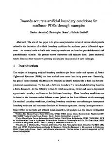
The 2D geometry consisted of a unit square (1m × 1m) with one elastic wall with thickness of 0.1 m. From the opposite side a parabolic velocity profile with mean velocity of 0.01 m/s was enforced. The third side had zero displacements and velocities and the fourth wall was a symmetry axis. The densities of the fluid and solid were both 1 kg/m3 , the viscosity was 1 Pas and the Young’s modulus 1 MPa. The time-step was 1 s and the calculation was continued until the computational mesh consisting of 240 bilinear elements was corrupted. The convergence criteria for determining the iteration for the current time-step was a relative change of 10−4 in the norm of all field variables. All in all 60 time-steps were computed. Convergence for each time-step was obtained after 12–19 coupled iterations as shown in Fig. 1. This must be considered to be quite a high number but in this case the coupling is pathological and the solution of the NavierStokes equation is not even possible without the scheme. The convergence history of the computed compressibility is shown in Fig. 2. Within each time-step the compressibility converges accurately to reflect the elastic strain of the moving wall. The fluid flux inside the square is 0.01 m2 /s. Therefore the volume as a function of time should be (1 + 0.01 t/s)m2 . This is compared to the computed volume in Fig. 4. The agreement is quite excellent even with this as the error in the end of the simulation is less than 0.1 %. Fig. 3 shows the computed compressibility as registered after each time step. The compressibility decreases gradually as the elastic strain increases. 5.2

3D case

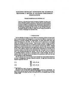
The 3D case was quite similar to 2D case. The geometry was extruded 1 m in the third dimension and the new boundaries were then given either symmetry boundary conditions or no-slip conditions. The material parameters were unaltered. The computational mesh was slightly sparser consisting of 1200 elements. In this case 39 time-steps could be computed before the mesh was corrupted. The convergence criteria was 10−3 for all field variables and convergence was obtained in 8–15 iterations. The relative error of the material conservation was slightly higher in this case, ranging up to 0.2 % as may be seen in Fig. 7. The computed compressibility has a similar behavior as in the 2D case, see Fig. 8. However, the absolute value is smaller by almost 7

Peter R˚ aback, Juha Ruokolainen, Mikko Lyly, and Esko J¨ arvinen

one order of magnitude which reflects the fact that the 3D structure is stiffer. Fig. 9 shows the deformed cube at 2, 20, 30 and 39 seconds. 6

CONCLUSIONS

In this paper an automated scheme for resolving the interaction between elastic structures and incompressible fluid was presented. The method is easily implemented as only the continuity equation requires some minor changes. The method gives good convergence in a very strongly coupled test case. In the trial runs it was noticed that small time-steps were more difficult to resolve. It seems therefore likely that the larger weight resulting from a small time-step may cause numerical problems. Even though the artificial compressibility has a physical basis it is still constrained by numerical considerations. In addition to the constant compressibility some alternatives for non-uniform compressibility were suggested. They have physically closer resemblance to the original phenomena of fluid-structure interaction since the compressibility may be limited to a thin layer at the interface. The test cases in this paper were very linear in nature and further tests are required to demonstrate the usability of the approach in a wider range of problems.

8

Peter R˚ aback, Juha Ruokolainen, Mikko Lyly, and Esko J¨ arvinen

REFERENCES [1] E. J¨arvinen, M. Lyly, J. Ruokolainen and P. R˚ aback. Three dimensional fluidstructure interaction modeling of blood flow in elastic arteries, Eccomas Computational Fluid Dynamics Conference, Swansea, 2001. [2] L. Formaggia, J. F. Gerbeau, F. Nobile and A. Quarteroni. Numerical treatment of defective boundary conditions for the Navier-Stokes equations, EPFL-DMA Analyse et Analyse Numerique, 20 (2000). [3] K. Riemslagh, J. Vierendeels, and E. Dick. An efficient coupling procedure for flexible wall fluid-structure interaction, Eccomas Congress on Comp. Meth. in Appl. Sci. and Eng., Barcelona, 2000. [4] A. J. Chorin. A Numerical method for solving incompressible viscous flow problems, J. Comput. Phys. 135, 118–125 (1997). [5] S. E. Rogers, D. Kwak and U. Kaul. On the accuracy of the pseudocompressibility method in solving the incompressible Navier-Stokes equations, Appl. Math. Modelling, 11, 35–44 (1987). [6] F. D. Carter and A. J. Baker. Accuracy and stability of a finite element pseudocompressibility CFD algorithm for incompressible thermal flows, Num. Heat Transfer, Part B, 20, 1–23 (1991). [7] ELMER finite element software homepage, http://www.csc.fi/elmer

9

Peter R˚ aback, Juha Ruokolainen, Mikko Lyly, and Esko J¨ arvinen

20

m

18 16 14 12 0

10

20

30 n

40

50

60

Figure 1: Number of fluid-structure iterations with time-step

−4

2.5

x 10

c (1/Pa)

2

1.5

1

0.5

0

50

100 i

150

200

Figure 2: Convergence history of the computed compressibility for 11 first time-steps

−3

10

−4

c (1/Pa)

10

−5

10

−6

10

0

0.1

0.2

0.3 dV/V

0.4

0.5

0.6

Figure 3: Computed compressibility with relative volume change

10

Peter R˚ aback, Juha Ruokolainen, Mikko Lyly, and Esko J¨ arvinen

−4

10

x 10

8

dV/V

6 4 2 0 −2

0

10

20

30 t (s)

40

50

60

Figure 4: Relative error of the material balance with iteration

Figure 5: The deformed geometry and velocity field after 2, 20, 40 and 60 seconds

11

Peter R˚ aback, Juha Ruokolainen, Mikko Lyly, and Esko J¨ arvinen

Figure 6: Computational mesh after 0 and 60 seconds

−3

2

x 10

dV/V

1.5

1

0.5

0

0

5

10

15

20 t (s)

25

30

35

40

Figure 7: Relative error of material balance with iteration in the 3D case

−4

c (1/Pa)

10

−5

10

−6

10

0

0.05

0.1

0.15

0.2 dV/V

0.25

0.3

0.35

0.4

Figure 8: Computed compressibility with relative volume change in the 3D case

12

Peter R˚ aback, Juha Ruokolainen, Mikko Lyly, and Esko J¨ arvinen

Figure 9: The deformed geometry at 2, 20, 30 and 39 seconds. The velocity is shown by vectors and colors on the elastic wall and on the two symmetry planes.

13