Flux boundary conditions in particle simulations

PHYSICAL REVIEW E 72, 026703 共2005兲

Flux boundary conditions in particle simulations 1

Eirik G. Flekkøy,1 Rafael Delgado-Buscalioni,2 and Peter V. Coveney3

Department of Physics, University of Oslo, P.O. Box 1048 Blindern, 0316 Oslo, Norway Departamento Ciencias y Técnicas Fisicoquímicas, Facultad de Ciencias UNED, Paseo del Rey 9, Madrid 28040, Spain 3 Centre for Computational Science, University College London, London WC1H 0AJ, United Kingdom 共Received 5 November 2004; revised manuscript received 31 May 2005; published 16 August 2005兲

2

Flux boundary conditions are interesting in a number of contexts ranging from multiscale simulations to simulations of molecular hydrodynamics in nanoscale systems. Here we introduce, analyze, and test a general scheme to impose boundary conditions that simultaneously control the momentum and energy flux into open particle systems The scheme is shown to handle far from equilibrium simulations. It acquires its main characteristics from the requirement that it fulfills the second law of thermodynamics and thus minimizes the entropy production, when it is applied to reversible processes. It is shown both theoretically and through simulations that the scheme emulates the effect of an extended particle system as far as particle number fluctuations, temperature, and density profiles are concerned. The numerical scheme is further shown to be accurate and stable in both equilibrium and far from equilibrium contexts. DOI: 10.1103/PhysRevE.72.026703

PACS number共s兲: 47.11.⫹j, 47.10.⫹g, 05.40.⫺a

I. INTRODUCTION

Both equilibrium and nonequilibrium particle simulations always require boundary conditions in addition to the prescription of the bulk dynamics. These boundary conditions may act to simulate an extended particle bath, as in standard equilibrium ensembles or a condition that maintains the system away from equilibrium as in a shear flow simulation. This is true whether the particle interactions are conservative as in a classical molecular dynamics simulation 关1兴, or dissipative as in dissipative particle dynamics 关2兴 or granular systems. While well-established techniques exist to introduce a pressure 关3兴 or a temperature 关4兴 in a nonlocal way, the present paper introduces local boundary conditions that allows the fluxes of momentum and energy to be simultaneously specified either as free parameters or in order to simulate an external reservoir. Such boundary conditions may be required in a wide variety of contexts where the hydrodynamic flow needs to be simulated on the molecular level, whether one studies imbibition in carbon nanotubes 关5兴, flows around proteins, or through layered liquid films 关6兴. Examples of such systems and processes also include temperature controlled, strong shears in nanolayers, or crossphenomena such as the thermomolecular effect in nanotubes 关7兴, and the osmotic flow of water through membranes 关8,9兴. Particle flux boundary conditions are interesting in particular for the design of multiscale simulation schemes where particle and continuum simulations are coupled by flux exchange algorithms 关10–14兴. For these schemes to be conservative the flux leaving one system must enter the other. In existing schemes the particle fluxes have been imposed by techniques that only produce the desired average fluxes, and are unstable or burdened with certain undesirable features 关15,16兴. The present scheme introduces the exact fluxes into the particle system. Moreover, it is analyzed and derived by a statistical mechanical argument. Our model is derived from the requirement that it be possible to impose reversible changes through the flux boundary 1539-3755/2005/72共2兲/026703共9兲/$23.00

conditions, i.e., that local equilibrium distributions be preserved and the entropy production minimized. From this it is shown how our algorithm may be used to perform molecular dynamics, or other particle simulations of systems which are governed by the grand canonical ensemble. Our approach differs from previous simulations using this ensemble 关17兴 by the use of open boundaries that connect to a reservoir of particles from which the flow of momentum and energy is controlled. Processes that are most effectively studied in the grand canonical ensemble include the equilibration of thin Black Newton films 关18兴, the swelling of clays in water 关19,20兴 or water between lamellar lipid structures 关21兴. We note that the scheme may also be applied to some nonstandard equilibrium ensembles. For instance, by setting the energy flux to zero and the momentum flux to a prescribed pressure p, an ensemble of fixed energy and pressure, but variable particle number N, may be simulated. In the present paper some simple 2D test simulations are carried out using soft sphere potentials, of both equilibrium and nonequilibrium processes. The scheme is shown to exhibit the predicted equilibrium behavior and remain both stable and accurate in far from equilibrium processes. The equilibrium behavior coincides with the theoretical predictions as far as density, temperature, and chemical potential profiles are concerned. Also, the energies are shown to satisfy the Boltzmann distribution and the particle number fluctuations reproduce the standard predictions of the grand canonical ensemble. The nonequilibrium processes examined include a freely expanding gas, in which case the model is shown to be both stable and numerically accurate, and shear flow simulations where the flow measurements agree with simple hydrodynamic predictions. The paper is organized as follows: In Sec. II the basics of the model are defined, In Sec. III the details are worked out and statistical mechanical arguments applied to derive the particle insertion and removal procedure. In Sec. IV the model is applied to simulate equilibrium ensembles, in Sec. V a numerical technique to improve accuracy is introduced, and in Sec. VI the simulation results are presented and dis-

026703-1

©2005 The American Physical Society

PHYSICAL REVIEW E 72, 026703 共2005兲

FLEKKOCSLY, DELGADO-BUSCALIONI, AND COVENEY

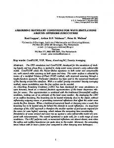
FIG. 1. Illustration of the model. The buffer is to the left of x = −xB and the nonconservative buffer force Fi acts only on the M = 16 particles there. At x = xB the particle velocities are reversed. In the vertical direction periodic boundary conditions are used.

cussed. Our conclusions are contained in Sec. VII. II. MODEL

It follows from Newton’s laws that it is impossible to prescribe the force on a body and the resulting velocity independently. For this reason we cannot simultaneously specify mass, momentum, and energy fluxes, and we choose to let the mass flux be the dependent quantity. For example, if our boundary conditions were applied at the ends of a pipe in which particles bounced back upon hitting the walls, the average mass flux would be determined by the pressure drop across the system, the net energy flux into it, as well as the shape of the pipe boundaries. A key feature of our model is the definition of a particle buffer where the fluxes are imposed, as illustrated in Fig. 1. In the present case the buffer is located to the left of the bulk particles at x ⬍ −xB where x is the horizontal coordinate. The buffer has a fixed number M of particles, while the overall particle number N 共which includes both bulk and buffer兲 will vary with time. Previous schemes have employed particle buffers too 关11–14兴, albeit with variable M. The fixed M prescription implies continuous particle creation and removal according to the flow between the region of bulk particles 共defined by x ⬎ −xB兲 and the buffer. Whenever a buffer particle crosses x = −xB a new particle is created in the buffer, and whenever a bulk particle crosses this boundary a buffer particle is removed. Here periodic boundary conditions are applied in the vertical direction, giving only one buffer cell. However, reflective boundary conditions could have been applied, or several neighboring buffer cells could have been introduced. The boundary conditions which are the topic of this paper are specified by the normal component of the energy flux j⑀ = j⑀ · n, where j⑀ is the energy flux and the normal component of the momentum flux j p = ⌸ · n, where ⌸ is the momentum flux tensor and n the unit normal shown in Fig 1. Both fluxes will in general include advective terms. The boundary conditions are intended to impose the exact momentum and energy flux to the whole N particle system, including the buffer. Since the buffer has a certain mass and

heat capacity the flux across the bulk boundary will both fluctuate and be somewhat delayed if j p and j⑀ depend on time. Correspondingly, the momentum and energy contained in the buffer will fluctuate. However, in real applications typically N ⬃ 104 or larger while M ⬃ 102 or smaller. The time scale of momentum and energy flow through the buffer will be correspondingly smaller than these time scales in the bulk. Hence the relative effect of the buffer mass and heat capacity will normally be negligible. The particle dynamics itself conserves mass, momentum, and energy. In the buffer zone there is an additional nonconservative force Fi. The average of this force will act to taper the particle density profile continuously to zero. The particle creation procedure is thus easily implemented as particles may be added in the dilute region away from other particles. While efficient techniques to add particles with the correct potential energy in dense particle systems do exist 关22兴, the present model circumvents any need for them. The flux boundary conditions introduce energy and momentum to the particle system both through the force Fi and particle addition/removal. We require that the combined effect is to create the prescribed momentum and energy fluxes, i.e., j pAdt = 兺 Fidt + 兺 ⌬共mvi⬘兲,

共1兲

j⑀ Adt = 兺 Fi · vidt + 兺 ⌬⑀i⬘ ,

共2兲

i⬘

i

i⬘

i

where i⬘ runs only over the particles that have been added or removed during the last time step dt, and A is the buffer-bulk interface area. The momentum change ⌬共mvi⬘兲 = mvi⬘ if the particle is added and ⌬共mvi⬘兲 = −mvi⬘ if the particle is removed. The energy change ⌬⑀i⬘ of the added/removed particles uses the same sign convention. The sums ⌺iFidt and ⌺iFi · vidt are the momentum and energy inputs due to Fi during the time dt. In order to simplify Eqs. 共1兲 and 共2兲 we define ˜j p and ˜j⑀ through the relations Adtj˜p = Adtj p − 兺 ⌬共mvi⬘兲 = 兺 Fidt,

共3兲

Adtj˜⑀ = Adtj⑀ − 兺 ⌬⑀i⬘ = 兺 Fi · vidt.

共4兲

i⬘

i⬘

i

i

Provided that the force Fi satisfies these conditions the correct energy and momentum fluxes into the particle system will result. III. STATISTICAL MECHANICS OF FLUX BOUNDARY CONDITIONS

In order to specify Fi and the particle addition/removal procedure we need a criterion in addition to Eqs. 共3兲 and 共4兲. This criterion is that it shall be possible to impose reversible changes to the system through the boundary conditions. This implies that the scheme must evolve the buffer via equilibrium states, or arbitrarily close to such states. In order for the

026703-2

PHYSICAL REVIEW E 72, 026703 共2005兲

FLUX BOUNDARY CONDITIONS IN PARTICLE SIMULATIONS

entire system to undergo reversible changes, momentum and energy must be added sufficiently slowly that the buffer and bulk have the time to equilibrate. To be more precise we introduce the Gibbs entropy S = − 兺 Pr log Pr ,

M

Fi · vi = MF · 具v典 + 兺 Fi⬘ · vi⬘ , 兺 i=1 i=1

Preq =

e −␤Er , Z

共5兲

共6兲

where Z is the partition function and Er = Ek + U共兵xi其兲, where U is the total potential energy, Ek = ⌺i共m / 2兲v⬘2i is the thermal kinetic energy, and ␤ is the Lagrange multiplier linked to the constraint ⌺rEr Pr = E. The velocity in Ek is the thermal comM vi / M. This ponent vi⬘ = vi − 具v典 where the average 具v典 = ⌺i=1 eq ensures Galilean invariance of Pr and that the entropy only depends on the thermal energy and not the overall translational energy of the buffer 关23兴. If any perturbation of the system brings the distribution away from its equilibrium form it will relax to equilibrium, spontaneously producing entropy, i.e., the process will be irreversible. The only way to achieve reversibility is to make sure the flux boundary scheme preserves the form of Preq at every step. First, we employ the following decomposition of the particle force Fi = F + Fi⬘ ,

Fi⬘ =

Aj˜p . M

冉 冊

1 1 mvi⬘2 = mvi⬘ · dvi⬘ = vi⬘ · Fi⬘dt ⬀ mvi⬘2 . 2 2

兺i=1 vi⬘2 M

关j˜⑀ − ˜j p · 具v典兴.

共11兲

This concludes the derivation of Fi. External particle forces that are proportional to the particle velocity have been widely applied and studied as heating mechanisms in molecular dynamics simulations 关24,25兴. However, to our knowledge such forcing schemes have not previously been generalized to control the momentum flux. The only thing that remains in order to define the full algorithm is to specify the particle addition/removal procedure. We start from the general observation that a factorized equilibrium distribution is easily preserved under the addition of a particle. The N-particle equilibrium distribution N peq simply becomes the N + 1-particle distribution ⌸i=1 i N+1 eq ⌸i=1 pi if the new particle is picked from the single particle distribution peq i . However, Preq is in general not factorizable. It may be written Preq = ⌳共兵xi其兲 兿 P MB共vi兲

共12兲

i

where the Maxwell-Boltzmann distribution

冉

P MB共vi兲 ⬀ exp

− 共m/2兲vi⬘2 T

冊

共13兲

when ␤ = 1 / T. As long as particle interactions cannot be neglected ⌳共兵xi其兲 will contain information on spatial correlations and will not factorize. Only in the low density limit will it do so. So, for the dilute end of the buffer we may write

共8兲

⌳共兵xi其兲 ⬀ 兿 ␳eq共xi兲,

共14兲

i

This implies that Fi⬘ gives no net momentum input, i.e., M Fi⬘ = 0, and that F does not alter the vi⬘’s. The latter fol⌺i=1 lows since the application of F over a time dt only changes the average velocity by changing all velocities vi by equal amounts. In particular, F has no effect on the distribution of 兵vi⬘其. The force Fi⬘ will preserve the form of the velocity distribution Peq共兵vi⬘其兲 ⬀ exp共−␤Ek兲 if its application over a time dt changes all the particle kinetic energies 共m / 2兲vi⬘2 by the same factor, i.e., d

Avi⬘

共7兲

where F alone satisfies Eq. 共3兲, i.e., F=

共10兲

which gives f and the particle force

r

where r = 兵xi , vi其i=1,…,N. Here and throughout we will work in units where kB = 1. In the absence of a Pauli principle this entropy is maximized for every N by the classical equilibrium distribution

M

共9兲

From this condition we obtain that Fi⬘ = fvi⬘ where the prefactor f may be determined from Eq. 共4兲. Note that while the distribution Peq共兵vi其兲 ⬀ exp共−␤Ek兲 keeps its form ␤ changes infinitesimally. The new ␤ is easily shown to be ␤⬘ = 关1 − 共2f / m兲dt兴␤. In order to determine f we use the identity

where ␳eq共xi兲 is the dilute limit of the equilibrium density profile and i now only runs over particles in the corresponding region. By adding particles with positions and velocities picked from the single particle distribution eq peq 0 共x,v兲 ⬀ ␳ 共x兲P MB共v兲,

共15兲

local equilibrium is preserved in the dilute part of the buffer. For global equilibrium to be preserved as well, we must again allow the system to remain sufficiently close to overall equilibrium states, so that the entropy production of the hydrodynamic modes following from the external fluxes remains negligible. In particular the heat conduction, which is likely to be the slower of the hydrodynamic modes, must be allowed to relax. Note that if we remove particles by randomly selecting them in the region where particles are added, the distribution of the removed particles is automatically the same as that of the added particles, i.e., Eq. 共15兲.

026703-3

PHYSICAL REVIEW E 72, 026703 共2005兲

FLEKKOCSLY, DELGADO-BUSCALIONI, AND COVENEY

The buffer density profile is easily predicted from the assumption of equilibrium. Since the buffer particle number M is fixed we may under equilibrium conditions write the average force on the buffer particles 具F典 as a potential force 具F典 =

pA n = − ⵱⌽, M

共16兲

where ⌽ = −pAx / M and p is a constant pressure. The fluctuations in F around the average 具F典 are caused by the particle insertion/removal and temperature fluctuations. In equilibrium the contributions from both these effects vanish. The potential ⌽ should then be considered as part of U and will thus act to define Preq. In equilibrium ␮ is constant throughout the system. We may thus write ␮ = ␮0(␳共x兲 , T) + ⌽共x兲 = const where ␮0 is the chemical potential at ␳共x兲 in the absence of any external potential. In the dilute part of the buffer we may use the ideal gas expression ␮0 = T0 log(␳共x兲 / ␳Q), where ␳Q is the quantum density. This gives the barometric density profile

␳eq共x兲 ⬀ e pAx/MT0 .

共17兲

The above result could also have been predicted from force balance arguments. In practice, it is an easy matter to observe where the profile acquires an exponential decay. In the simulations particle insertion/removal is carried out at x ⬍ −3xB which is well within this domain, and the spatial probability distribution for particle insertion is normalized to unity over this region. Since both particle addition and removal are reversible in the sense that they minimize the entropy production we may write the entropy change associated with the addition of ⌬N particles as T⌬S⬘ = 兺 ⌬⑀i⬘ − ␮⌬N.

共18兲

i⬘

This is the standard form of the second law when the volume available to the system is not changed. But the total entropy change to the system during the time ⌬t, during which the ⌬N particles are added, also includes the heating due to Fi⬘. For isolated systems 共⌬N = 0兲 it has been shown both analytiM cally and through simulations 关24兴 that T⌬S = ⌺i=1 Fi⬘ · vi⬘⌬t. Hence since particle addition and the application of Fi⬘ happen sequentially we may assume the following additive form for the entropy change: M

T⌬S = T⌬S⬘ + 兺 Fi⬘ · vi⬘⌬t.

共19兲

i=1

Combining this result with the expression for the corresponding energy change M

M

⌬E = 兺 Fi · vi + 兺 ⌬⑀i⬘ = MF · 具v典⌬t + 兺 Fi⬘ · vi⬘⌬t i⬘

i=1

+ 兺 ⌬ ⑀ i⬘ i⬘

we obtain

i=1

共20兲

T⌬S = ⌬E − ␮⌬N − MF · 具v典⌬t.

共21兲

We define the volume change ⌬V of the system as A times the buffer center of mass displacement in the x direction, i.e., ⌬V = − A具v典 · n⌬t.

共22兲

By using Eq. 共16兲 to eliminate An we get p⌬V = − MF · 具v典⌬t,

共23兲

and we obtain the standard form of the second law for reversible processes T⌬S = ⌬E + p⌬V − ␮⌬N.

共24兲

Finally, we note that the existence of the barometric density profile Eq. 共17兲 requires a positive pressure. Indeed, the existence of a dilute region relies on this. With a positive external pressure p the existence of a finite equilibrium vapor pressure will guarantee some ideal gas region where x Ⰶ −xB and the local pressure drops to zero 关27兴. However, with a negative pressure, as may, for instance, occur in water in narrow conduits, the present algorithm will not work and must be replaced by schemes that add particles in dense regions 关22,26兴. Theoretically, it is not known how the imposition of the exact energy flux or preservation of local equilibrium may be achieved in these cases, although as shown in Ref. 关22兴, the system relaxes to the expected equilibrium state within a few collision times if the correct amount of potential energy is released upon each particle insertion.

IV. APPLICATIONS AND EQUILIBRIUM ENSEMBLES

The model may now be applied in various ways. As mentioned already it solves the problem of flux imposition in hybrid schemes where j⑀ and j p are provided as time dependent boundary conditions by some continuum solver. As a means to simulate equilibrium ensembles the boundary condition most naturally realizes the grand canonical ensemble. By taking j⑀ = −␭共T − T0兲 where ␭ is a relaxation parameter that plays the role of a heat conductivity, and the temperature is defined by the relation T = 具mv2 / 2典, we simulate a heat bath of temperature T0. By setting j p = np we fix the pressure p. The freely adjustable particle number N will then equilibrate around an average that is governed by the chemical potential ␮共p , T0兲. The bulk part of the system which has fixed volume also has fixed external T0 and ␮, and is thus described by the grand canonical ensemble. Other choices are of course possible too. By setting j⑀ = 0, p fixed and specifying the Maxwell-Boltzmann distribution for the added particles by the internal temperature T, one defines an ensemble where energy and pressure are fixed but where N and T are fluctuating. Likewise, one could fix the enthalpy H of the total system by setting j⑀ = M具v典 · F, or equivalently ⌬E + p⌬V = ⌬H = 0. However, the system is still open, so this choice does not correspond to an insulated system. Hence these two latter ensembles may be of theoretical interest only as it is unclear how one would realize them experimentally.

026703-4

PHYSICAL REVIEW E 72, 026703 共2005兲

FLUX BOUNDARY CONDITIONS IN PARTICLE SIMULATIONS V. ACCURACY ENHANCEMENT AND STABILITY OF THE FLUX BOUNDARY SCHEME

Particle addition and removal cannot be done in a simple way without causing discontinuous jumps in Fi. While this is not a problem in principle it reduces the numerical accuracy of the scheme. In order to smooth these jumps and improve the numerical accuracy we introduce the reservoir variables, ⌬Pr and ⌬Er for momentum and energy. The idea is that when a particle is removed or added the corresponding momentum and energy correction is returned to the system gradually, rather than in a single punch. For this purpose the following fluxes are defined to enter in Eqs. 共8兲 and 共11兲 ˜j p = j p − ⌬Pr and ˜j⑀ = j⑀ − ⌬Er , ␶r A ␶r A

共25兲

where ␶r is a time scale larger than dt but smaller than any relevant hydrodynamic time scale. The momentum and energy added to the particles from the reservoir variables over a time step dt are −⌬Prdt / ␶r and −⌬Erdt / ␶r, respectively. Correspondingly, these variables are updated according to the rules ⌬Pr → ⌬Pr − ⌬Pr

dt + 兺 ⌬共mvi⬘兲, ␶r i ⬘

⌬Er → ⌬Er − ⌬Er

dt + 兺 ⌬ ⑀ i⬘ . ␶r i

However, this is not a major problem, and even far from equilibrium simulations are stable and converge to equilibrium, as is described below. The parameter ␭ sets the time needed to relax the buffer to any desired value of T0. The simulations described below were all stable and the choice of ␭ corresponds to a relaxation time smaller than a few ␶’s, and thus corresponds to relatively strong heating/cooling. Finally, if j⑀ and j p are set to maintain a state for which j⑀ ⬍ 具v典 · j p, i.e., where the overall energy input is less than the work done by j p, the system will be unstable. The physical reason is that more energy is extracted than added, and the thermal velocities will decay to zero. Physical considerations would normally exclude such a boundary condition.

共26兲

VI. SIMULATIONS

In these simulations Newtons second law is integrated using the velocity-Verlet algorithm and an interparticle potential U共r ⬍ d兲 = 共k / 2兲共d − r兲2 where d is the particle diameter, r the center separation, and k a spring constant. The simulation domain includes a bulk particle region at −xB ⬍ x ⬍ xB and −y max ⬍ y ⬍ y max. At y = ± y max periodic boundary conditions are applied and at x = xB the particles bounce back with reversed velocities, thus conserving energy. In the simulations the length unit is the particle diameter d and the unit of time the inverse frequency 冑m / k associated with the potential. This implies the unit kd2 for energy. The velocity Verlet scheme is as follows:

⬘

Initially, ⌬Pr and ⌬Er are both 0. While the scheme of Eqs. 共3兲 and 共4兲 leads to fixed momentum and energy fluxes into the system, the present scheme delays the compensation of the momentum and energy input associated with particle addition/removal by a characteristic time ␶r. If no more particles are added or removed ⌬Pr and ⌬Er will decrease exponentially on the time scale ␶r. Hence the variables ⌬Pr and ⌬Er act to smooth Fi as a function of time while the total momentum and energy input instead become 共slightly兲 discontinuous with particle addition/removal. If we set ␶r = dt we recover the original scheme and the actual fluxes will again exactly equal the prescribed ones. What are the stability criteria of the above algorithm? Two types of instabilities have been observed, one linked to overheating at the dilute end of the system, and one associated with the effect of cooling the system below the available thermal energy. Since the mean free time ␶ that controls the relaxation rate to local equilibrium increases with decreasing density, it will become large at the far end of the buffer region where the density is low. Since Fi⬘ ⬀ vi⬘ hot particles here may become increasingly hot and escape due to lack of equilibration. If this happens the distribution of Eq. 共15兲 breaks down and the velocity distribution becomes position dependent. This problem may be dealt with by increasing M. When the magnitude of j ⑀ may be chosen at will, say by changing ␭ in our case, one may also decrease j⑀ thus lowering the heating per particle.

ri共t + ⌬t兲 = ri共t兲 + vi⌬t +

Fi共t兲 2 ⌬t + o共⌬t3兲, 2m

冉 冊 兲 冉 冊 vi t +

⌬t Fi共t兲 ⌬t, = vi共t兲 + 2 2m

vi共t + ⌬t = vi t +

Fi共t + ⌬t兲 ⌬t ⌬t + o共⌬t3兲. + 2 2m

共27兲

This is the standard scheme 关4兴. Note, however, that since Fi depends not only on position but also on velocities we have to use Fi共t + ⌬t兲 = Fi„兵r j共t + ⌬t兲其,兵v j + 共1/m兲F j共t兲⌬t其…

共28兲

in order to get third order accuracy in vi共t + ⌬t兲. In summary the model is implemented by the repeated performance of the following three steps. 1. Propagate the particle positions and velocities using Eq. 共28兲 with the current values of F and Fi⬘ given by Eqs. 共8兲 and 共11兲. 2. Update the momentum and energy reservoirs, Eqs. 共26兲, and the fluxes ˜j p and ˜j⑀, Eq. 共25兲. 3. Update the forces Eqs. 共8兲 and 共11兲 and return to 1. First, the stability and accuracy of the scheme is tested. Every simulation was started with particles in the buffer zone only, and then the system was left to relax. Initially, a fixed j⑀ = 0.5 was applied and then replaced by j⑀ = −␭共T − T0兲 with ␭ = 0.5. Figure 2 shows the relaxation of such a free expan-

026703-5

PHYSICAL REVIEW E 72, 026703 共2005兲

FLEKKOCSLY, DELGADO-BUSCALIONI, AND COVENEY

FIG. 4. The relative error in energy after t = 400 as a function of M when ␭ = 0.5, ␶r = 1.

FIG. 2. Snapshots of a free expansion simulation at t = 0, 10, 30, 50, and 70 where initially only the buffer zone contained particles. The error in energy is given as a fraction of the total energy. Here xB = −12, M = 200, dt = 0.02, p = 1.0, ␭ = 1.0, T0 = 0.5, and ␶r = 1.

sion simulation where initially there were only 共randomly placed兲 particles in the buffer. The stability of such a freely expanding system is of interest for the study of shock fronts. The error in energy ␦E is defined as the difference between the measured energy, which includes ⌬Er, and the prediction E0 + 兰dtAj⑀, where E0 is the initial energy. Figures 3 and 4 show the resulting error after t = 400 as functions of dt and M, respectively. When dt 艌 0.01 the error scales roughly as dt3. When dt ⬍ 0.01 the round-off errors appear to dominate. The variations with M are small down to the M = 64 value below which the heat capacity of the buffer starts to become too small to accommodate the variations in the flux j⑀. In Fig. 5 we have plotted the density and temperature profiles throughout the buffer region. The solid line represents a best fit to an exponential in the buffer region. Due to the presence of interactions between particles, this fitted curve decays somewhat more slowly than the low density profile of Eq. 共17兲. However, in the dilute tail of the curve the measured decay rate of ␳共x兲 agrees well with the prediction of Eq. 共17兲. In the ␳ ⬍ 0.1 region the discrepancies between the predicted decay coefficient in the exponential, pA / 共MT0兲, and the measured one were smaller than 5%. The result of Fig. 5 is less obvious than it may appear. The fact that the temperature is roughly constant throughout the buffer and bulk particle region, and that the density falls off exponentially in the buffer region is drastically changed if the particle addition/removal scheme is changed. For in-

FIG. 3. The relative error in energy after t = 400 as a function of dt when ␭ = 0.5, ␶r = 1, and M = 200. The dashed line has slope 3.

FIG. 5. The particle density ␳共x兲 共䊊兲 and temperature T共x兲 共䉭兲 as a function of −x. The full line shows a best fit to an exponential in the buffer region. The profile was averaged over time 500⬍ t ⬍ 4000. Except for the value xB = −6 parameters are as in Fig. 2.

026703-6

PHYSICAL REVIEW E 72, 026703 共2005兲

FLUX BOUNDARY CONDITIONS IN PARTICLE SIMULATIONS

FIG. 6. The time-averaged pressure as a function of time at the rightmost wall, x = xB divided by the imposed P = j p · n, corresponding to the simulation in Fig. 2. The dashed line shows the instantaneous pressure, averaged only over the time dt while the full line shows the corresponding running average over a time window ⌬t = 50. The straight line is the expected value.

stance, by inserting and removing particles at different average energies, or at different average locations, the profiles are significantly changed. The results of Figs. 4 and 5, which show the numerical accuracy and the proximity of equilibrium in the simulations, dictate the choice of M. These results reflect what is happening in the buffer, so this choice does not depend on the number of bulk particles. In practice one needs M ⬎ 60. Figure 6 shows the results of measuring the pressure as function of time. The pressure is measured as the momentum change per unit area per unit time at the right hand wall where particles are subject to the bounce back condition. When averaged the pressure is indeed seen to conform to the imposed value. The initial overshoot is associated with the free-expansion phase before the system reaches equilibrium. Figure 7 shows the local distributions of kinetic energy. The curves in Fig. 7 are averaged over sections of the buffer region. The lowest curve corresponds to an average over particles located at −50⬍ x + xB ⬍ −40, the next curve to particles in −40⬍ x + xB ⬍ −30 and so forth to the upper curve which is obtained from particles in −10⬍ x + xB ⬍ 0. The probabilities are not normalized by the local density, hence the shift between the curves directly corresponds to the decrease in ␳共x兲, which is almost two orders of magnitude less

FIG. 7. The probability Px共EK兲 of finding the kinetic energy EK as a function of EK for different values of x 共䊊兲. The straight lines are linear fits. Here xB = −6 and the other parameters are as in Fig. 2.

FIG. 8. The temperature as a function of density. T0 = 0.5 and T / T0 are the slopes in Fig. 7 in the buffer region.

for the lower than for the upper curve. It is seen from Fig. 7 that T0 log共Px共EK兲兲 = const − EK

共29兲

to a good approximation, i.e., that the Boltzmann distribution Px共EK兲 ⬀ exp共−EK / T0兲 is satisfied locally. To quantify this statement the slopes of the curves in Fig. 7 are plotted in Fig. 8. The expected slopes are −1, while the actual slopes measure −T0 / T where T is the local temperature. The local value of T does not fluctuate significantly beyond expected equilibrium fluctuations. It is reassuring that the system is well equilibrated even within the low density tail as the consistency of the model relies on this property. Figure 9 shows the particle number as a function of time. In the very first stages t 艋 50, there is a rapid increase in N共t兲 as the system fills up with particles. After the free expansion phase a density wave and hydrodynamic oscillations in N共t兲 are seen. After t = 500 the wave that is caused by the filling process decays and we are left with the equilibrium fluctuations. To investigate whether the flux boundary conditions really play the role of an extended particle system, we measure the fluctuations in N at constant T0. According to the standard of statistical mechanics 关23兴 具⌬N2典 = 共N − M兲T

冏 冏 ⳵␳ ⳵p

,

共30兲

T

where N − M is the bulk particle number. In the ideal gas limit this reduces to 具⌬N2典 = N − M, which is the result we

FIG. 9. The particle number N as a function of time. Except for the value xB = −6 parameters are as in Fig. 2.

026703-7

PHYSICAL REVIEW E 72, 026703 共2005兲

FLEKKOCSLY, DELGADO-BUSCALIONI, AND COVENEY

FIG. 10. The number fluctuations 共䊊兲 as a function of pressure p at a temperature T0 = 0.5 and M = 200. The theoretical prediction 共䉭兲 is based on equation of state measurements, and the full line shows a polynomial fit to these.

expect for low pressures. For higher pressures the repulsive interparticle potential is felt and 具⌬N2典 ⬍ N − M. In an independent set of measurements using periodic boundary conditions in all directions the constant temperature equation of state p = p共␳兲 was measured. From these measurements ⳵␳ / ⳵ p兩T was obtained, both from finite differencing the p共␳兲 data and from the derivative of a polynomial fit to p共␳兲. In Fig. 10 具⌬N2典 / 共N − M兲 is compared to T⳵␳ / ⳵ p兩T. It is seen that the fluctuations conform to the prediction within the noise which is intrinsic both to the equation of state measurements and the measurements of 具⌬N2典. In other words, as far as particle number fluctuations go the effect of our flux boundary conditions is the same as that of an extended particle system. Finally, we briefly examine the case where there is a shear imposed on the system. Figure 11 shows a shear flow where the average velocity reaches the thermal velocity over a few mean free paths. The velocity profile is quite linear within the bulk particle region as one would expect from hydrodynamics. Also the buffer density profile is still close to exponential, and the temperature profile roughly constant as in equilibrium. Interestingly the particle number fluctuations 具⌬N2典 共not shown兲 have decayed to half the equilibrium value in these nonequilibrium simulations.

FIG. 11. Shear flow simulation: The density ␳ 共full line兲, temperature T 共䉭兲, and velocity uy共x兲 共䊐兲 as a function of position. The momentum flux j p = 1.5ex + 0.1ey where ex and ey are the unit vectors in the x and y directions. The average is taken over the time interval 500⬍ t ⬍ 4000, M = 200, ␭ = 0.5, T0 = 0.5, and the final energy error is roughly 1%.

bination of a buffer force and particle addition/removal, and it may be used to impose any thermodynamic state on the particle system, both at and away from equilibrium. This algorithm and the fact that it closely approximates a particle reservoir when applied to reversible processes is the main outcome of the paper. The algorithm may be used in conjunction with continuum solvers to carry out hybrid computations of far from equilibrium processes where no adequate continuum description exists, for instance, transitions to boundary shear localization, the moving contact line, or the molecular hydrodynamics around nanostructures. The present simulation scheme has been shown to be stable and accurate to less than 1% in errors of energy in all 2D simulations studied here, both near and far from equilibrium. The scheme can easily be generalized to 3D by the simple replacement T → 共3 / 2兲T for the average kinetic energy. Work is in progress to implement the present scheme in hybrid simulations that hitherto have lacked an accurate scheme for flux imposition which maintains the particle domain in a close to equilibrium state. ACKNOWLEDGMENTS

We have proposed a scheme that has been used to impose arbitrary energy and momentum fluxes across the boundaries of an open particle system. This scheme relies on the com-

It is a pleasure to thank Renaud H. Toussaint and Knut Jørgen Måløy for helpful comments. This research was partly supported by the EPSRC RealityGrid project grant GR/ R67699. R. D.-B. also acknowledges support from project BFM2001-0290.

关1兴 B. Alder and T. Wainwright, Phys. Rev. Lett. 18, 968 共1970兲. 关2兴 P. J. Hoogerbrugge and J. M. V. A. Koelman, Europhys. Lett. 19, 155 共1992兲. 关3兴 D. A. Anderson, Computational Fluid Dynamics 共McGrawHill, Singapore, 1995兲. 关4兴 M. Allen and D. Tildesley, Computer Simulations of Liquids 共Clarendon Press, Oxford, 1987兲.

关5兴 S. Supple and N. Quirke, Phys. Rev. Lett. 90, 214501 共2003兲. 关6兴 T. Becker and F. Mugele, Phys. Rev. Lett. 91, 166104 共2003兲. 关7兴 S. de Groot, Thermodynamics of Irreversible Processes 共North-Holland, Amsterdam, 1952兲. 关8兴 T. Ito and T. Yamaguchi, J. Am. Chem. Soc. 126, 6202 共2004兲. 关9兴 E. G. Flekkøy, J. Feder, and T. Jøssang, J. Stat. Phys. 68, 515 共1992兲.

VII. CONCLUSIONS

026703-8

PHYSICAL REVIEW E 72, 026703 共2005兲

FLUX BOUNDARY CONDITIONS IN PARTICLE SIMULATIONS 关10兴 S. T. O’Connell and P. A. Thompson, Phys. Rev. E 52, R5792 共1995兲. 关11兴 E. G. Flekkøy, G. Wagner, and J. G. Feder, Europhys. Lett. 52, 271 共2000兲. 关12兴 R. Delgado-Buscalioni and P. V. Coveney, Phys. Rev. E 67, 046704 共2003兲. 关13兴 E. G. Flekkøy, J. Feder, and G. Wagner, Phys. Rev. E 64, 066302 共2001兲. 关14兴 S. Barsky, R. Delgado-Buscalioni, and P. V. Coveney, J. Chem. Phys. 121, 2043 共2004兲. 关15兴 G. Wagner and E. G. Flekkøy, Philos. Trans. R. Soc. London, Ser. A 362, 1 共2004兲. 关16兴 R. Delgado-Buscalioni and P. V. Coveney, Philos. Trans. R. Soc. London, Ser. A 362, 12 共2004兲. 关17兴 J. Ji, T. Cagin, and B. M. Pettitt, J. Chem. Phys. 96, 1333 共1992兲. 关18兴 J. Faraudo and F. Bresme, Phys. Rev. Lett. 92, 236102 共2004兲.

关19兴 A. A. Bowden, P. Boulet, P. V. Coveney, and A. Whiting, J. Mater. Chem. 13, 2540 共2003兲. 关20兴 E. S. Boek, P. V. Coveney, and N. T. Skipper, J. Am. Chem. Soc. 117, 12608 共1995兲. 关21兴 A. V. Broukhno, Ph.D. thesis, Lund University, 2003. 关22兴 R. Delgado-Buscalioni and P. V. Coveney, J. Chem. Phys. 119, 978 共2003兲. 关23兴 L. D. Landau and E. M. Lifshitz, Statistical Physics 共Pergamon Press, New York, 1959兲. 关24兴 N. G. Hadjiconstantinou, Phys. Rev. E 59, R44 共1999兲. 关25兴 H. J. C. Berendsen et al., J. Chem. Phys. 81, 3684 共1984兲. 关26兴 G. D. Fabritiis, R. Delgado-Buscalioni, and P. V. Coveney, J. Chem. Phys. 121, 12139 共2004兲. 关27兴 We note that with strong interparticle attraction the number of molecules in the dilute vapor region may also become impractically small in parts of the pT phase space of the LennardJones liquid.

026703-9