Fock space multireference coupled cluster calculations based on an underlying bivariational self-consistent field on Auger and shape resonances Y. Sajeev, Manoj K. Mishra, Nayana Vaval, and Sourav Pal Citation: J. Chem. Phys. 120, 67 (2004); doi: 10.1063/1.1630025 View online: http://dx.doi.org/10.1063/1.1630025 View Table of Contents: http://jcp.aip.org/resource/1/JCPSA6/v120/i1 Published by the American Institute of Physics.
Additional information on J. Chem. Phys. Journal Homepage: http://jcp.aip.org/ Journal Information: http://jcp.aip.org/about/about_the_journal Top downloads: http://jcp.aip.org/features/most_downloaded Information for Authors: http://jcp.aip.org/authors
Downloaded 01 Mar 2012 to 59.162.23.79. Redistribution subject to AIP license or copyright; see http://jcp.aip.org/about/rights_and_permissions
JOURNAL OF CHEMICAL PHYSICS
VOLUME 120, NUMBER 1
1 JANUARY 2004
Fock space multireference coupled cluster calculations based on an underlying bivariational self-consistent field on Auger and shape resonances Y. Sajeev Theory Group, Physical Chemistry Division, National Chemical Laboratory, Pune 411 008, India
Manoj K. Mishra Department of Chemistry, Indian Institute of Technology, Powai, Mumbai 400 076, India
Nayana Vaval and Sourav Pala) Theory Group, Physical Chemistry Division, National Chemical Laboratory, Pune 411 008, India
共Received 1 August 2003; accepted 8 October 2003兲 The Fock space multireference coupled cluster based on an underlying bivariational self-consistent field is applied to the problem of computing complex energy associated with Auger and shape resonances in e-atom scattering. It is concluded that the Fock space multireference coupled cluster based on a bivariational self-consistent field provides a useful and practical approach to calculation of resonance parameters. Numerical results are presented for the 2P shape resonance of Mg and Auger 1 s⫺1 hole of Be. © 2004 American Institute of Physics. 关DOI: 10.1063/1.1630025兴
I. INTRODUCTION
Though conceptually simple, difficulties may arise in treating molecular systems using complex scaling method.6 Introduction of an absorbing boundary condition in the exterior region of the molecular scattered target using a complex absorbing potential 共CAP兲7 may be an alternative and numerically simpler route to solve resonance of the molecules. CAP potentials have been applied to molecules in the context of configuration interaction and electron propagator techniques.8 A complex self-consistent field 共SCF兲9 technique, also called bivariational SCF,10,11 has been attempted to calculate many electron atomic or molecular resonances. In these calculations the resonance energies and width are calculated as a difference between the ground state total energies of the (N⫾1) and the neutral target. The total energy of the ion is stabilized with respect to scale parameter while the total energy of the neutral target is assumed to be stable for ⫽1.0. The resonant energy eigenvalues were obtained by a SCF method in a manner very similar to standard SCF technique. Mishra et al.12 showed that a crude approximation of the resonance eigenvalues can be deduced using Koopmans’ theorem once the complex energies for all orbitals are obtained. The ionization potential/electron affinity studies using Koopmans’ theorem provided with the simultaneous calculation of both energy 共real part兲 and width 共twice the imaginary part兲 of electron detachment Auger resonance (E N0 – E sN⫺1 ) and electron attachment shape resonance (E sN⫹1 – E N0 ), where s labels a stationary state and E N0 is the ground state total energy of the neutral N electron target. In this case, any stabilization is attributed to the total energies of the corresponding N⫾1 system. The resonance eigenvalues obtained by the Koopmans’ theorem can always be modified by correlation studies. The role of correlation and relaxation in the formation and decay of metastable states has been reported.13 The ac-
The resonances are characterized by the complex energy eigenvalues Z⫽E⫺i⌫/2, where E gives the position of the resonance and ⌫ gives the width of the resonance.1 The corresponding eigenfunctions diverge asymptotically and do not belong to the Hermitian domain of the Hamiltonian. The dilation of atomic Hamiltonian has emerged as a practical and potentially accurate method for the calculation of resonance parameters in electron–atom scattering.2– 4 These methods are based on the mathematical developments of several workers.5 The essential idea in these methods to the resonance problem is to make a transformation on Hamiltonian which results in a non-Hermitian operator, one of the square integrable eigenfunctions of which corresponds to the resonant state. The associated complex eigenvalue then gives the position and width of the resonance or auto-ionizing state. The dilation transformation of the electronic coordinate r→r , where is a complex number, is used to make the resonance function square integrable. In atomic physics, in which particles are interacting with coulomb forces, the transformation r→r is quite straightforward. For arg() larger then some critical values, the complex eigenvalues correspond to the resonance Z⫽E⫺i⌫/2 of H( ), are invariant to change, i.e., d nZ ⫽0; dn
n⫽1,2.... .
共1兲
The advantage of this method over complex continuum calculations is that the resonance eigenfunctions are square integrable and thus many existing electronic structure calculation for the bound state can be adapted to the resonance. a兲
Author to whom correspondence should be addressed. Electronic mail:
[email protected]
0021-9606/2004/120(1)/67/6/$22.00
67
© 2004 American Institute of Physics
Downloaded 01 Mar 2012 to 59.162.23.79. Redistribution subject to AIP license or copyright; see http://jcp.aip.org/about/rights_and_permissions
68
Sajeev et al.
J. Chem. Phys., Vol. 120, No. 1, 1 January 2004
curacy of the SCF approximations in the case of an electron scattering resonance depends on the extent to which the electron correlation is important in the description of particular states. This can be achieved by an effective Hamiltonian, which corrects for the inadequacies of the bivariationaly obtained Hartree–Fock operator. Thus complex SCF calculations on resonance will provide the best starting point for more accurate calculations. The Fock space multireference coupled cluster 共FSMRCC兲14 –16 method has been quite successful in the calculation of electron affinity and ionization potential. In this paper, we formulate a FSMRCC method based on the complex SCF for the first time to the direct and correlated calculations of resonance energy and width. This can describe the dynamic and nondynamic electron correlation efficiently in the ionized or electron attached states. The MRCC method is based on a prechosen model space and the main ionizations can be conveniently described using a model space of important (N⫺1) electron determinants and an appropriate exponential wave operator to describe the dynamic electron correlation. Diagonalization of an effective Hamiltonian17 over the model space provides the multiple roots of the state. Using the restricted Hartree–Fock of the N electron system as vacuum, the (N⫺1) electron determinants constitute onehole Fock space. Similarly with one-particle model space, electron affinity can be determined. The Bloch effective Hamiltonian18 has been used quite successfully in the FSMRCC method to describe ionization potential, electron affinity, and excitation energies. Quite clearly, a complex scaled FSMRCC can be a potentially powerful candidate to compute resonance energies and the width of the resonances. In this paper we present resonant parameters and optimal scaling values obtained by the FSMRCC method. The 1 s⫺1 hole in Be leads to a KLL Auger resonance and has been studied both experimentally and theoretically.12,19,20共a兲,20共b兲 The 2P shape resonance in e-Mg scattering serves as a problem for checking the theoretical scheme for the treatment of shape resonance and has been studied extensively.9,21,22 We have utilized 共10s/6p兲 contracted Gaussian-type orbitals 共CGTO兲10 and 共14s/11p兲 CGTO23共a兲 bases for Be and a 共4s/ 9p兲 CGTO23共b兲 base for Mg since other theoretical results are available in these bases. Section II contains a brief outline of the bivariational SCF method which serves as a starting point of our MRCC method to compute the resonance. In Sec. III we will develop the FSMRCC technique to compute resonance energy and a trajectory method to singling out the resonance orbital. In Sec. IV we will present our results for the calculation of the 1 s⫺1 Auger hole in Be and 2P shape resonance in Mg. Further improvement in the characterization of the resonance using MRCC methods is presented in Sec. V. II. BIVARIATIONAL SCF
In the complex self-consistent field method 共bivariational SCF兲 proposed by Mishra et al.,10 a complex Hamiltonian was used together with real basis functions. The difference between the usual Hartree–Fock theory and bivariational SCF is that in the latter, the energies of various
orbitals are now complex. For the complex values of the dilation parameter , the dilated atomic Hamiltonian H共 兲⫽
兺i
冉
冊
1 2 2 Z 1 ⵜi ⫺ ⫹ ; 2 ri r i⬍ j ij
兺
⫽ ␣ e ⫺i 共2兲
is non-Hermitian, and therefore variational theorem does not apply. However, a bivariational theorem for non-Hermitian operators can be applied and the bivariational SCF equations for the complex scaled Hamiltonians are derived by extremizing the generalized functional 共 ⌽ 0 ,⌿ 0 兲 ⫽ 具 ⌽ 0 兩 H 共 兲 兩 ⌿ 0 典 / 具 ⌽ 0 兩 ⌿ 0 典 .
共3兲
The trial functions ⌽ 0 and ⌿ 0 are built from linearly independent one-particle functions or spin orbitals ⌽ 0 ⫽ 共 N! 兲 ⫺1/2 det兵 i 共 x i 兲 其 ,
共4兲
⌿ 0 ⫽ 共 N! 兲 ⫺1/2 det兵 j 共 x j 兲 其 ,
共5兲
where the indices i and j go from 1 to N. The sets 兵 I 其 1M and 兵 I 其 N1 (M ⭓N) of spin orbitals are biorthonormal
具 i兩 j 典 ⫽ ␦ i j .
共6兲
Extremization of the functional in Eq. 共3兲 results in the following SCF equations: F i ⫽ i i ,
共7a兲
F ⫹ i ⫽ * i i ,
共7b兲
where 1 F 1 共 , , 兲 ⫽⫺ 2 ⵜ 21 ⫺ Z/r 1 2 ⫹
冕
1⫺ p 12 共 x 2 ⬘ ,x 2 兲 dx 2 , x 2 ⬘ ⫽x 2 r 12
共8兲
occ
⫽
兺i i *i .
共9兲
The complex symmetry nature of the dilated Hamiltonian H ⫹ ( )⫽H * ( ) suggests the dual choice of basis ⌽ and ⌿ having the property ⌽⫽⌿ * and the consequent association 兵 i 其 ⫽ 兵 * i 其 to make the approximate manyelectron wave function satisfy same relation as the exact one. The advantages of this assumption 兵 i 其 ⫽ 兵 i* 其 and the details of the implementation of the bivariational SCF procedure are given in Ref. 10. A. Fock space MRCC method to calculate resonance
We choose the restricted Hartree–Fock determinant for N electron as the vacuum. With respect to this vacuum, holes and particles are defined. Depending on the energies of interest, these are further divided into active and inactive sets such that each determinant I of the model space has at least one active particle. For an (N⫹1)/(N⫺1) electron state, the model space consists of determinants consisting of one active particle/hole. These are called one-particle or one-hole model space. The active particles or holes can be so defined as to make the model space complete.
Downloaded 01 Mar 2012 to 59.162.23.79. Redistribution subject to AIP license or copyright; see http://jcp.aip.org/about/rights_and_permissions
J. Chem. Phys., Vol. 120, No. 1, 1 January 2004
⌿ 0 共 1,0兲 ⫽
兺 c i⌽ i , i苸ap
SCF on Auger and shape resonance
共10兲
where 共1,0兲 denotes one active particle and zero active holes present in the model space determinants 兵 I 其 . C i are the model space coefficients. The exact wave function can be written in the Fock space method using Lindgren’s normal ordered ansatz16 as ⌿ 共1,0兲 ⫽⍀⌿ 共0 兲共 1,0兲 , ˜
⍀⫽ 兵 e T 共 1,0兲 其 ,
共11兲 共12兲
where ⍀ is a valence-universal wave operator, and the curly bracket denotes an operator within it to be normally ordered. The valence universality of the wave operator ensures connectivity and size extensivity of the Fock space Bloch equations. To ensure this, ˜T (1,0) is defined to contain the amplitudes for lower valence sectors too. Hence the Ts used are capable of describing the problem consisting of lower valence electrons. ˜T 共 1,0兲 ⫽T 共 0,0兲 ⫹T 共 1,0兲 ,
共13兲
(0,0)
is only a hole-particle creation operator and the where T T (1,0) operator destroys exactly one valence particle in the model space. Each of these Ts can be written as the sum of different n-body operators. If the one-body scaling term is introduced in the Hartree–Fock level, the Fock space MRCC theory has a complex vacuum and consequently the complex molecular orbitals dictates that the T operator for all the sectors will be complex. T 共 0,0兲 ⫽
兺n T 共n0,0兲 ,
共14a兲
T 共 1,0兲 ⫽
兺n T 共n1,0兲 .
共14b兲
To calculate the electron affinity, we substitute the wave function into the Schrodinger equation for the multiple roots of the (N⫹1) electron states. The roots are obtained as eigenvalues of the effective Hamiltonian17 defined over the model space. The model space and the wave operator ⍀ are obtained by the Bloch equation18 projected to the 共1,0兲 model space as well as its lower sector, in this case 共0,0兲 sector H 共eff1,0兲 C⫽CE,
共15兲
Q 共 m,n 兲 H⍀ P 共 m,n 兲 ⫽Q 共 m,n 兲 ⍀H effP 共 m,n 兲 ᭙m⫽0,1
᭙n⫽0
共16兲
P 共 m,n 兲 H⍀ P 共 m,n 兲 ⫽ P 共 m,n 兲 ⍀H effP 共 m,n 兲 ᭙m⫽0,1
᭙n⫽0.
共17兲
The eigenvalues of the H eff’s, E s, are the exact energies of the system. Equations for cluster amplitudes are solved using the subsystem embedding condition, i.e., first equations for the lowest sector are solved. With the Ts of the lower sectors as constants, equations for higher Fock space sectors are solved progressively upwards. Normal ordering and the subsystem embedding condition together decouple
69
the equations for each Fock space sector. The solution of the Bloch equation defines the effective Hamiltonian over the model space. It has dimensions the same as model space dimensions and eigenvalues correspond to the exact energies of the system, i.e., electron affinity 共E.A.兲 of the system. The vacuum expectation value of the effective Hamiltonian is the energy of the closed shell N electron state or zero-valence problem. Diagrammatically, this can be dropped easily and the eigenvalues of the resultant effective Hamiltonian of one valance Fock space sector provide us with direct difference energies. However, the effective Hamiltonian is a complex non-Hermitian matrix, in general. In a similar manner, we can solve the MRCC equations for the 共0,1兲 sector of the model space and can carry out the ionization potential 共IP兲 calculations. In this paper, we have used a singles and doubles approximation for the cluster amplitudes of both zero and one valence sector. This FSMRCCSD approximation has been noted to be quite accurate for the purpose of IP/E.A. calculation. However, one may note that in the FSMRCC method of computing direct difference energies, the energy of the ground state is computed with the scaled Hamiltonian. This is a result of the direct evaluation of the difference energies. The dependence of the electron affinity/ ionization potential as well as the ground state energy with the scaling parameter is worth investigating. We may note that the dependence on the scaling parameter is a feature with all methods, which obtain these difference energies in a direct manner. The dependence of the scaling parameter is, however, a manifestation of the finite basis set as will be discussed in the next section.
B. The trajectory method for resonant energies and width by the E.A.ÕIP search
Several workers5 have studied the transformations of the spectrum of the Hamiltonian for an N⫹1 particle system under complex scaling. The spectrum is transformed in such a way that the resonance states become isolated in the complex energy plane. Based on these spectrum transformation ( )⫺E N results, the EA⫽E N⫹1 n 0 obtained from MRCC calculations may be classified as follows. 共1兲 Bound state eigenvalues and scattering thresholds are invariant of and if n denotes a bound state E n N⫹1 ( ) is ( )⫺E N⫹1 is a persistent real and persistent. Therefore E N⫹1 n 0 real energy. 共2兲 As continua rotate as a function of , complex eigenvalues may be exposed. These eigenvalues are independent of as long as they are isolated from the continuum. These complex energies correspond to resonances. If n denotes a ( )⫽E rN⫹1 resonant 共metastable state兲 of the ion, E N⫹1 n ⫺i⌫/2 and the corresponding energy difference E N⫹1 () n N⫹1 N ⫽(E ( )⫺E )⫺i⌫/2 gives the position 共real part兲 ⫺E N 0 r 0 and half width 共imaginary part兲 of the resonances. A similar analysis may be carried out for the ionization potential to calculate the position and width of Auger resonance. With this brief discussion of the calculation of energy differences as a common background, its utility in direct and simultaneous treatment of resonances of N⫾1 electron systems becomes manifest.
Downloaded 01 Mar 2012 to 59.162.23.79. Redistribution subject to AIP license or copyright; see http://jcp.aip.org/about/rights_and_permissions
70
Sajeev et al.
J. Chem. Phys., Vol. 120, No. 1, 1 January 2004
FIG. 1. trajectory(10s/6p basis兲 for the Auger 1 s⫺1 hole in Be. ␣ ⫽0.85 and increments are in the steps of 0.02 rad. The values begin with 0.0 rad for the Im E⫽0.0 eV. SCF共—䊐—兲; FSMRCC共—䊊—兲.
While the EA/IP corresponding to the resonance is persistent once uncovered and should be invariant to further changes in the complex scaling parameter, applications employing the manageable basis sets do not fulfill the condition d k Z/d k ⫽0
᭙k⫽1,2,3,... .
共18兲
This condition for total stability is instead seen to manifest itself as quasistability in the short range of . The stability of resonance is then examined through the following relation:
Z/ ⫽0
共19兲
and for ⫽ ␣ e ⫺i one has the reciprocity relations 共 Z/ 兲 ␣ opt⫽⫺i 共 Z/ 兲 ⫽0
共20a兲
共 Z/ ␣ 兲 opt⫽i / ␣ 共 Z/ 兲 ⫽0.
共20b兲
and Equation 20共a兲 can be solved by plotting trajectory, which is a graphical method in which resonance energy Z is plotted as a function of , holding ␣ fixed. In a similar way Eq. 20共b兲 can also be solved. The stationary points along the trajectories which satisfy the complex form of virial theorem correspond to slowing down 共closing of distance between consecutive points兲 or cusps of these trajectories. The tedious and expensive graphical solution of Eq. 共20兲 is the principal bane of complex coordinate calculations. III. RESULTS AND DISCUSSION
FIG. 2. trajectory(10s/6p basis兲 for the Auger 1 s⫺1 in Be. increments are in the steps of 0.02 rad. The values begin with 0.0 rad for the Im E ⫽0.0 eV. ␣ ⫽0.80(—䊊—); ␣ ⫽0.85(—䊐—); ␣ ⫽0.90(—䉭—); ␣ ⫽0.95(—⫻—).
are shown in Fig. 2. The slowing down accompanied by a small cusp is seen in the trajectories for ␣ ⫽0.90 and 0.95. To determine the optimal value of alpha we next examine the alpha trajectories 共Fig. 3兲 for ⫽0.08, 0.09, and 0.10 rad. These trajectories display a coalescence of the points near the ␣ ⫽0.90 and this value of alpha is taken as the optimal value. After the optimal point, the trajectories show monotonous increase of distance between the consecutive points. The values for the energy and width obtained by various theoretical and experimental methods are shown in Table I. Our results also show a good agreement with these results. We have done similar calculations using the 14s/11p basis set. The alpha trajectories for these calculations are shown in Fig. 4. The optimum value of the scaling parameters ( ␣ opt ⫽0.75– 0.78, opt⫽0.26 rad) for this basis set is different from that of 10s/6p basis used. The results we got using this higher basis set is closer to the experimental result and higher order dilated-propagator theory results. The trajectories plotted by using higher basis sets are more stable than that of a lower basis set and show less dependence of scaling parameters near the resonant point. B. 2P shape resonance in Mg
The shape resonances belong to the continua attached to the first threshold of the target and are easiest to analyze. The alkaline earth element Mg has a P-type orbital as the lowest unoccupied orbital. These p orbitals are ideally suited for
A. The 1 sÀ1 Auger hole in Be
The 1 s⫺1 Auger hole in Be is studied by checking the ionization potential calculations using the FSMRCC method for various scaling parameters. A comparative study of trajectories between the uncorrelated SCF and FSMRCC for the ␣ ⫽0.85 is shown in Fig. 1 using the 10s/6p basis set. The noticeable difference between the two trajectories shows the need for the inclusion of correlation and relaxation in the study of Auger resonances. It is seen that by including the correlation, the energy is lowered. This can be due to the additional screening of the nucleus by other electrons. The positive imaginary part coming in the bivariational SCF level away from the optimum values of the scaling parameter may be due to the instability of complex SCF and use of finite basis set. The trajectories for ␣ ⫽0.80, 0.85, 0.90, and 0.95
FIG. 3. ␣ trajectory(10s/6p basis兲 for the Auger 1 s⫺1 hole in Be. ␣ increments are in steps of 0.2. The trajectories starts from the right for the ␣ value⫽1.00 ⫽0.07 rad(—䊊—); ⫽0.08 rad(—䊐—); ⫽0.09 rad(—䉭—); ⫽0.10 rad(—⫻—).
Downloaded 01 Mar 2012 to 59.162.23.79. Redistribution subject to AIP license or copyright; see http://jcp.aip.org/about/rights_and_permissions
J. Chem. Phys., Vol. 120, No. 1, 1 January 2004
SCF on Auger and shape resonance
TABLE I. Energy and width of Be⫹ (1 s⫺1 ) 2S Auger resonance. Energy 共eV兲
Method Experimenta Many body perturbation theoryb Second order dilated electron propagatorc Quasiparticle diagonal 2ph-TDA dilated electron propagatord Zeroth order dilated electron propagatord Second order electron propagator with Siegert boundary conditione Third order decoupling of dilated electron Propagator (14s/11p basis兲f Fock space MRCC based on bivariational SCF 共this work兲 10s/6p basis 14s/11p basis
71
TABLE II. Energy and width of 2P shape resonance in e-Mg scattering.
Width 共eV兲
Method a
123.63 124.98
0.09 0.05
127.90
0.54
128.80
0.24
125.47
0.02
124.63
0.76
126.97 123.82
0.38 0.45
a
Reference 24. Reference 19. c Reference 25. d Reference 26. e Reference 20共a兲. f Reference 23共a兲. b
providing centrifugal angular momentum barrier of adequate width and depth to temporarily trap the impinging electron. We have performed a series of calculations with different values of scaling parameter alpha and theta on this system, which employs a 4s/9p basis of real valued Gaussian functions. The results obtained from experiment and various theoretical methods and for e-Mg scattering are collected in Table II. Our result for energies and width are in good agreement with experimental and other theoretical methods. In a MRCC calculation using the complex Hamiltonian H( 兵 r 其 ), there is a stationary behavior of the complex electron affinity with respect to variation of the theta and alpha to be expected; at some value of and ␣, E/ and E/ ␣ vanishes, respectively. However, in calculations utilizing limited basis sets only quasistability in a narrow region of alpha and theta values is observed. The resonances are identified by plotting the complex electron affinity as a function of theta 共theta trajectory兲 for alpha values near the optimal values and the
FIG. 4. ␣ trajectories(14s/11p basis兲 for the Auger 1 s⫺1 hole in Be. ␣ increments are in steps of 0.02. The trajectories start from the bottom part for the initial value of ␣ ⫽0.62. ⫽0.24 rad(—䊊—); ⫽0.26 rad(—䊐—); ⫽0.29 rad(—䉭—).
Experiment Static exchange phase shiftb Static exchange plus polarizability phase shiftb Static exchange cross sectionc Static exchange plus polarizability cross sectionc S-matrix pole 共x alpha兲d Second order biorthogonal Dilated electron propagatore Complex SCF.f Configuration interactionf Fock space MRCC calculation based on bivariational SCF 共this work兲
Energy 共eV兲
Width 共eV兲
0.15 0.46 0.16
0.13 1.37 0.24
0.91 0.19
2.30 0.30
0.08 0.15
0.17 0.13
0.51 0.20 0.13
0.54 0.23 0.18
a
Reference 27. Reference 28. c Reference 29. d Reference 30. e Reference 31. f Reference 32. b
quasistable region in the trajectory is associated with resonance energy 共real part兲 and half width 共imaginary part兲; the same way alpha trajectories are also constructed for theta values near the optimal values. The lowering of both the energy and width near the stationary point in the theta trajectories shown in Figs. 5 and 6 seems to indicate that relaxation of the target helps the impinging electron to see more nuclear attraction 共lower energy兲, whereby it spends more time in the vicinity of the target 共has smaller width兲. This is reflected in our MRCC calculations by the cusp near the stationary points in the trajectories. MRCC calculations also shows some of the notable features of the stabilization method33 that at the point of optimal stabilization of the resonant root there is an avoided crossing with another nearly degenerate root which descends from above and replaces the stabilization root when further changes in the stabilization parameter are affected. The two theta trajectories in Fig. 7 correspond to two different scattering root approaches to each other from the opposite direction in the complex energy plane and there is almost an
FIG. 5. The trajectories for the 2P shape resonance in Mg⫺ . Initial value of ⫽0.02 rad and its starts from the top. increments are in the steps of 0.02 rad. The average value near the converged points is marked as ␥. ␣ ⫽0.72(—䉭—); ␣ ⫽0.73(—䊐—); ␣ ⫽0.75(—䊊—).
Downloaded 01 Mar 2012 to 59.162.23.79. Redistribution subject to AIP license or copyright; see http://jcp.aip.org/about/rights_and_permissions
72
Sajeev et al.
J. Chem. Phys., Vol. 120, No. 1, 1 January 2004
The basic purpose of our work is to use a highly correlated Fock space MRCC method using complex scaling to compute ionization potential/electron affinity, and thus to provide a method to obtain more accurate energy and width of the resonance. Our results show the correlation and relaxation effects in the calculation of resonance. ACKNOWLEDGMENT
The authors thank the Department of Science and Technology 共DST兲, New Delhi, for financial support towards this work. FIG. 6. Variation of real共E兲 and imaginary共E兲 with respect to : ␣ ⫽0.72(—䉭—); ␣ ⫽0.73(—䊐—).
avoided crossing near the resonance. These trajectories correspond to different orbitals and display an identical resonance behavior near the crossing point. The wave packet nature of the incoming electron beam can explain the multiple resonant roots. The key idea of the stabilization theory is that the resonances are localized inside the potential barrier. The wave packet is made up of many waves falling within the width of the packet center. As such, orbital bases of the kind employed here with nearly degenerate orbital energies in close proximity to the resonance energy will give rise to different roots describing the different roots of the packet whose width is determined by the width of the widest root. The optimum value of ␣ ( ␣ opt⫽0.72– 0.75) is the same as that of the dilated electron propagator calculation21 which is also based on an underlying bivariational SCF. But our MRCC method needs a larger rotation to uncover resonance( opt propagator ⫽0.26– 0.30 rad, opt ⫽0.12 rad). This may be due to the high theta dependency of the ground state energy of the n electron target E n ( opt). IV. CONCLUDING REMARKS
The electron correlation and relaxation effects play a substantial role in the formation and decay of resonance. The description of the resonance energy levels at the bivariational SCF level is included only to discriminate that the correlation and relaxation effects characterizes the resonance.
FIG. 7. The trajectories for multiple resonant roots. Root I 共—䊐—: ␣ initial⫽0.7, ␣ increment⫽0.01) starts from bottom right and root II 共—䉭—: ␣ initial⫽0.65, ␣ increment⫽0.01) starts from top right.
W. P. Reinhardt, Annu. Rev. Phys. Chem. 33, 323 共1982兲. B. R. Junker, Adv. At. Mol. Phys. 18, 207 共1982兲. 3 Y. K. Ho, Phys. Rep. 99, 2 共1983兲. 4 Int. J. Quantum Chem. 共1978兲, Vol. 4 is devoted entirely to complex scaling and more references therein. 5 E. Balslev and J. M. Combes, Commun. Math. Phys. 22, 280 共1971兲; J. Aguilar and J. M. Combes, ibid. 22, 269 共1971兲; B. Simon, ibid. 27, 1 共1972兲; Ann. Math. 97, 247 共1973兲. 6 C. W. McCrudy, Autoionization: Recent Developments and Applications, edited by A. Tempkin 共Plenum, New York, 1985兲, pp. 153–170. 7 U. V. Riss and H.-D. Meyer, J. Phys. B 26, 4503 共1993兲; R. Santra and L. S. Cederbaum, J. Chem. Phys. 115, 6853 共2001兲. 8 R. Santra and L. S. Cederbaum, J. Chem. Phys. 117, 5511 共2002兲; S. Feuerbacher, T. Sommerfeld, R. Santra, and L. S. Cederbaum, J. Chem. Phys. 118, 6188 共2003兲; T. Sommereld, U. V. Riss, H.-D. Meyer, L. S. Cederbaum, B. Engels, and H. U. Suter, J. Phys. B 31, 4107 共1998兲. 9 C. W. McCurdy, T. N. Rescigno, E. R. Davidson, and J. G. Lauderdale, J. Chem. Phys. 75, 1835 共1981兲. 10 ¨ hrrn, and P. Froelich, Phys. Lett. 84A, 4 共1981兲. M. Mishra, Y. O 11 P. Froelich and P. O. Lowdin, J. Math. Phys. 24, 88 共1983兲. 12 ¨ hrrn, J. Chem. Phys. 79, 5494 共1983兲. M. Mishra, O. Goscinski, and Y. O 13 N. Moiseyev and F. Weinhold, Phys. Rev. A 20, 27 共1979兲. 14 R. Offerman, W. Ey, and H. Kummel, Nucl. Phys. A 273, 349 共1976兲; R. Offerman, ibid. 273, 368 共1976兲; W. Ey, ibid. 296, 189 共1978兲. 15 D. Mukherjee and S. Pal, Adv. Quantum Chem. 20, 291 共1989兲; S. Pal, M. Rittby, R. J. Brtlett, D. Sinha, and D. Mukherjee, J. Chem. Phys. 88, 4357 共1988兲; U. Kaldor and M. A. Haque, Chem. Phys. Lett. 128, 45 共1986兲; U. Kaldor and M. A. Haque, J. Comput. Chem. 8, 448 共1987兲; D. Mukherjee, Pramana 12, 1 共1979兲; A. Haque and D. Mukherjee, J. Chem. Phys. 80, 5058 共1984兲. 16 I. Lindgren, Int. J. Quantum Chem. S12, 33 共1978兲; J. Phys. B 24, 1143 共1991兲; Phys. Scr. 32, 291 共1985兲; I. Lindgren and D. Mukherjee, Phys. Rep. 151, 93 共1987兲; W. Kutzelnigg, J. Chem. Phys. 77, 2081 共1982兲; W. Kutzelnigg and H. Koch, ibid. 79, 4315 共1983兲. 17 P. Durand and J. P. Malrieu, Adv. Chem. Phys. 67, 321 共1987兲; J. P. Marlrieu, P. L. Durand, and J. P. Daudey, J. Phys. A 18, 809 共1985兲. 18 C. Bloch, Nucl. Phys. A6, 329 共1958兲. 19 H. P. Kelly, Phys. Rev. A 11, 556 共1975兲. 20 共a兲 M. Palmquist, P. L. Altick, J. Richter, P. Winkler, and R. Yaris, Phys. Rev. A 23, 1787 共1981兲; 共b兲 P. Bisgard, R. Bruch, P. Dahl, and M. Rodbro, Phys. Scr. 17, 1931 共1978兲. 21 ¨ hrn, J. Chem. Phys. 79, M. Mishra, H. A. Kurtz, O. Goscinski, and Y. O 1896 共1983兲. 22 C. W. McCurdy, J. G. Lauderdale, and R. C. Mowrey, J. Chem. Phys. 75, 1835 共1981兲. 23 共a兲 A. Venkitnathan, S. Mahalakshmi, and M. K. Mishra, J. Chem. Phys. 114, 35 共2001兲; 共b兲 R. A. Donnelly, ibid. 76, 5414 共1982兲. 24 P. Bisgard, R. Bruch, P. Dahl, B. Fatrup, and M. Rodbro, Phys. Scr. 17, 49 共1978兲; M. Robro, R. Bruch, and P. Bisgard, J. Phys. B 12, 2413 共1979兲. 25 ¨ hrn, J. Chem. Phys. 79, 5505 共1983兲. M. Mishra, O. Goscinski, and Y. O 26 M. N. Medikeri and M. Mishra, Adv. Quantum Chem. 27, 223 共1996兲. 27 P. D. Burrow, J. A. Michejda, and J. Comer, J. Phys. B 9, 3255 共1976兲. 28 ¨ hrn, Phys. Rev. A 19, 43 共1979兲. H. A. Kurtz and Y. O 29 H. A. Kurtz and K. D. Jordan, J. Phys. B 14, 4361 共1981兲. 30 P. Krylstedt, N. Elander, and E. J. Brandas, J. Phys. B 21, 3969 共1988兲. 31 M. N. Medikeri, J. Nair, and M. Mishra, J. Chem. Phys. 99, 1869 共1993兲. 32 A. U. Hazi, J. Phys. B 11, L259 共1978兲. 33 H. S. Taylor, Adv. Chem. Phys. 18, 91 共1970兲. 1 2
Downloaded 01 Mar 2012 to 59.162.23.79. Redistribution subject to AIP license or copyright; see http://jcp.aip.org/about/rights_and_permissions