3Physics Department, Brooklyn College, CUNY, Brooklyn, New York 11210. 4Laboratoire ... guess for the wave function; in addition, it benefits from the. Brillouin ...
PHYSICAL REVIEW A, VOLUME 66, 012504
Coupled-cluster calculations using local potentials C. Gutle´,1 J. L. Heully,2 J. B. Krieger,3 and A. Savin4 1
Laboratoire de Chimie The´orique, CNRS and Universite´ Pierre et Marie Curie, F-75252 Paris, France 2 Laboratoire de Physique Quantique, Univerite´ Paul Sabatier, F-31062 Toulouse, France 3 Physics Department, Brooklyn College, CUNY, Brooklyn, New York 11210 4 Laboratoire de Chimie The´orique, CNRS and Universite´ Pierre et Marie Curie, F-75252 Paris, France 共Received 28 December 2001; revised manuscript received 19 March 2002; published 19 July 2002兲 Coupled-cluster calculations starting from exchange-only local-density approximation 共XLDA兲, Krieger-LiIafrate 共KLI兲, and Kohn-Sham 共KS兲 wave functions are compared with those using the Hartree-Fock 共HF兲 determinant as a reference. The total energies are found to be close, the difference being maximally 2 mhartree in the systems studied 共the first terms in the He, Be, Ne, Mg, Ar isoelectronic series兲. The convergence is, however, sensitive to the choice of the reference: KLI and KS converge, in general, faster than HF in spite of being a worse approximation in the first two orders of perturbation theory. The improvement of convergence due to the use of the KLI or KS references is more pronounced in the systems showing near degeneracy, such as in the Be series. For XLDA, the convergence properties are either comparable to those of KLI or oscillatory, depending on the system. In a second part, the numerical results are analyzed 共in the HF and KLI cases兲 by using first-order developments with respect to nuclear charge Z at large Z. DOI: 10.1103/PhysRevA.66.012504
PACS number共s兲: 31.25.Eb, 31.15.Dv, 31.15.Md, 02.60.Cb
I. INTRODUCTION
Usually, many-body calculations are performed using the Hartree-Fock operator as a single-particle reference, since this method yields the energetically lowest one-determinant guess for the wave function; in addition, it benefits from the Brillouin theorem as a technical simplification. However, it is well known that Hartree-Fock 共HF兲 orbitals very poorly describe excited states. Kelly 关1兴 has recognized the importance of the choice of virtual orbitals in calculating the correlation energy, and proposed to use the Hartree-Fock orbitals of the system with one electron removed. Davidson 关2兴 has further analyzed the role of the virtual orbitals in perturbation theory by partitioning differently the Hamiltonian such that the reference Hartree-Fock determinant is rotated through unitary transforms. Alternatively, the Kohn-Sham 共KS兲 potential seems to have a convenient ordering of virtual states 共see, e.g., 关3兴兲. It has been proposed by Fritsche 关4兴 to use the KS wave function as a reference for correlated calculations. This choice ensures, in addition, the exact density at zeroth order. Go¨rling and Levy 关5兴 developed a perturbation theory for the correlation energy, where the external potential is constrained to keep the ground-state density correct at each order. The KS potential is, however, not known in general. As a first approximation to it, it seems reasonable to use the optimized effective potential 共see, e.g., the work of Talman and Shadwick 关6兴, or more recently Engel and coworkers 关7,8兴兲, or the Krieger-Li-Iafrate 共KLI兲 关9兴 approximation to this exact-exchange potential 共see, e.g., Engel et al. 关10兴 for application to molecules兲. Exact-exchange Kohn-Sham methods 关11兴 have been used too. Moreover, using the KLI potential is consistent with density-functional theory schemes if we prospect further for methods coupling wave function with density 关12兴. Shankar and Narasimhan 关13,14兴 have performed correlated calculations using orbitals obtained in the X ␣ local approximation. More recently, calculations have been performed using approximate density1050-2947/2002/66共1兲/012504共14兲/$20.00
functional potentials 关15,16兴. X ␣ and KLI potentials are quite different in the asymptotic region, the first decaying exponentially, the last proportional to 1/r 共for neutral systems兲. Thus, the virtual orbitals are expected to be quite different in the two approximations. In preceding papers 关17,18兴, we made preliminary calculations at the level of second order perturbation theory using KLI and KS orbitals in Slater basis sets. In the present paper, we go further with numerical coupled-cluster calculations using singly and doubly excited states 共CCSD兲 and compare the results obtained starting with orbitals from the exchangeonly local-density approximation 共XLDA兲 and KLI method to those obtained with HF orbitals. When possible, comparisons with KS wave functions were also made. The final part of the paper discusses the dependence of the correlation energy upon the nuclear charge Z 共in the large Z limit兲 and upon the choice of the unperturbed system 共HF, KLI兲. Concerning the second point, we noticed a difference of sensitivity upon the potential in the approximation used 共CCSD or second-order of perturbation theory兲. We would like to point out that the problem mentioned by Bonetti et al. 关19兴 is of no importance here: while they use second-order perturbation theory to construct a local potential, we make correlated calculations starting with a given potential. II. COUPLED-CLUSTER CALCULATIONS A. Technical details
The systems under investigation here are chosen to be closed-shell atoms and their first isoelectronic cations because accurate numerical calculations in that field are feasible, using the nonrelativistic CCSD program by Salomonson and co-workers 关20兴. Furthermore, the behavior of these series with nuclear charge Z is known from Linderberg and Shull 关21兴 and finally we possess very precise estimations of the exact correlation energies by Chakravorty et al. 关22兴 to be compared with.
66 012504-1
©2002 The American Physical Society
C. GUTLE´, J. L. HEULLY, J. B. KRIEGER, AND A. SAVIN
PHYSICAL REVIEW A 66, 012504 共2002兲
FIG. 1. Second-order and coupled-cluster correlation energies E c as a function of the nuclear charge Z. Thin line, second order; thick line, coupled clusters; full line, He series (Z苸 关 2,11兴 ); long dashed line, Be series (Z苸 关 4,13兴 ); dashed line, Ne series (Z苸 关 10,20兴 ); dashed dotted line, Mg series (Z苸 关 12,23兴 ); dotted line, Ar series (Z苸 关 18,27兴 ). Note that in the HF case, the second-order and coupled-cluster curves are almost indistinguishable at the scale of the figure, except for the Be series. Same remark for the He series in the KLI case.
The HF and XLDA potentials are obtained from the nonrelativistic self-consistent-field program 关23兴, and the KLI potentials from the Li program 关24兴. The KS potentials were generated by Colonna and co-workers 关25,26兴 共in the He and Be series兲 and Filippi et al. 关27兴 共for the neon atom兲. In the numerical coupled-cluster program 关20兴, we included all the single and double excitations giving nonzero contributions in a multipole expansion of 1/r 12 as a sum of spherical harmonics products up to angular momentum l ⫽14. We used 200 orbitals per symmetry so that the valence and Rydberg states are well described, as we expected the KLI potential to produce more bounded states than the HF potential does. The potentials were projected on an exponential grid of a thousand points scaled with the nuclear charge Z and the number of electrons in the system. We expect for our results the numerical accuracy of a few tenths of mhartrees in the He, Be, and Ne series and 1 mhartree in the Mg and Ar series. They are given without radial or angular extrapolations as we estimate this effect to be below 0.1 mhartree and thus irrelevant for the purpose of our paper, which is the comparison between different potentials. B. Energies
In this section, we present our results for the energies and correlation energies. First, we comment on the effect of changing the nuclear charge in a series 共system-specific point of view兲 while keeping the same variant of potential 共HF, XLDA, KLI, or KS兲 for the calculations. Then we specify to a given system and vary the type of potential 共referencespecific point of view兲. Some general trends are noted, to be commented in Sec. III 共when HF and KLI potentials are used兲 with the help of a simplified model developed for that purpose. 1. System-specific point of view
In Fig. 1, the HF and KLI correlation energies E c are plotted with respect to nuclear charge Z, both at second-order
perturbation theory and CCSD levels. At large Z, we observe that the correlation energies are nearly constant with Z in the He and Ne series and linearly decreasing in the Be, Mg and Ar series. This behavior was expected for the exact correlation energy from Linderberg and Shull 关21兴. We find it here still valid in the approximations of second-order perturbation theory and coupled cluster. Furthermore, it is valid whatever the choice of the unperturbed Hamiltonian 共HF, XLDA, and KLI兲. More precisely, in case of linearity 共Be, Mg, Ar series兲, the slopes are ordered Be⬎Ar⬎Mg. 2. Reference-specific point of view
The numerical results are reported in Tables I and II for the He and Be series, respectively. Ne, Mg, and Ar series are available as supplementary data in Ref. 关34兴. If we consider a given system in one of these tables, the first row deals with HF reference, the second with XLDA, the third with KLI, and the fourth with KS reference 共if the KS potential was available兲. a. Energies of the references. The second column specifies the expectation values of the Hamiltonian (E HF , E XLDA , E KLI , or E KS ) with different determinants 共HF, XLDA, KLI, or KS, respectively兲 to be compared now. We expected E HF to be smaller or equal to E XLDA , E KLI , and E KS by definition. In fact E HF and E KLI are found relatively close. E HF ⫽E KLI in the He series 关9兴; for the cases studied, we pointed out differences (E KLI ⫺E HF ) up to 1 mhartree in the Be series, of 23 mhartree in the Ne series 共we will present the results as xy, where x corresponds to the beginning of the series, and y to the end兲, 45 mhartree in the Mg series, and 78 mhartree in the Ar series. A slight increase of E KLI ⫺E HF with nuclear charge is present; it is however expected to disappear as Z→⬁. E KS ⫺E HF is larger than E KLI ⫺E HF . It is probably due to a constraint of exact density added to that of locality (E KS ⫺E HF is 0.030.07 mhartree in the He series, 212 mhartree in the Be series兲. This difference has been used by Valderrama et al. 关28兴 to define
012504-2
PHYSICAL REVIEW A 66, 012504 共2002兲
COUPLED-CLUSTER CALCULATIONS USING LOCAL . . .
TABLE I. Total energies in the He series 共a.u.兲. Consider a given nuclear charge 共Z兲 in the first column. We present the 共monodeterminantal兲 first-order energy (E V ) in the second column, the second-order energy (E V(2) ) in the third column, the third-order energy (E V(3) ) in the fourth column, the coupled-cluster energy (E CCSD(V) ) in the fifth column, and an estimation of the exact total energy (E exact ) 关22兴 in the sixth column. V specifies the potential used for the calculation: V⫽HF in the first row, XLDA in the second row, KLI in the third row 共and KS in the fourth row when it was available兲. Z
EV
E V(2)
E V(3)
E CCSD(V)
E exact
2 共HF兲 共XLDA兲 共KLI兲 共KS兲
⫺2.8617 ⫺2.8578 ⫺2.8617 ⫺2.8616
⫺2.8990 ⫺2.9125 ⫺2.9100 ⫺2.9101
⫺2.9009 ⫺2.9053 ⫺2.9056 ⫺2.9056
⫺2.9037 ⫺2.9037 ⫺2.9037 ⫺2.9037
⫺2.9037
3
⫺7.2364 ⫺7.2330 ⫺7.2364 ⫺7.2364
⫺7.2766 ⫺7.2851 ⫺7.2839 ⫺7.2840
⫺7.2780 ⫺7.2814 ⫺7.2813 ⫺7.2813
⫺7.2799 ⫺7.2799 ⫺7.2799 ⫺7.2799
⫺7.2799
4
⫺13.6113 ⫺13.6080 ⫺13.6113 ⫺13.6113
⫺13.6530 ⫺13.6592 ⫺13.6585 ⫺13.6586
⫺13.6541 ⫺13.6567 ⫺13.6566 ⫺13.6566
⫺13.6556 ⫺13.6556 ⫺13.6556 ⫺13.6556
⫺13.6556
5
⫺21.9862 ⫺21.9830 ⫺21.9862 ⫺21.9862
⫺22.0289 ⫺22.0338 ⫺22.0333 ⫺22.0333
⫺22.0298 ⫺22.0319 ⫺22.0318 ⫺22.0318
⫺22.0310 ⫺22.0310 ⫺22.0310 ⫺22.0310
⫺22.0310
6
⫺32.3612 ⫺32.3580 ⫺32.3612 ⫺32.3612
⫺32.4045 ⫺32.4086 ⫺32.4082 ⫺32.4082
⫺32.4053 ⫺32.4070 ⫺32.4070 ⫺32.4069
⫺32.4062 ⫺32.4062 ⫺32.4062 ⫺32.4062
⫺32.4062
7
⫺44.7362 ⫺44.7330 ⫺44.7362 ⫺44.7361
⫺44.7799 ⫺44.7834 ⫺44.7831 ⫺44.7831
⫺44.7806 ⫺44.7821 ⫺44.7821 ⫺44.7820
⫺44.7814 ⫺44.7814 ⫺44.7814 ⫺44.7814
⫺44.7814
8
⫺59.1111 ⫺59.1080 ⫺59.1111 ⫺59.1111
⫺59.1552 ⫺59.1583 ⫺59.1580 ⫺59.1580
⫺59.1559 ⫺59.1572 ⫺59.1571 ⫺59.1571
⫺59.1566 ⫺59.1566 ⫺59.1566 ⫺59.1566
⫺59.1566
9
⫺75.4861 ⫺75.4830 ⫺75.4861 ⫺75.4861
⫺75.5305 ⫺75.5332 ⫺75.5330 ⫺75.5330
⫺75.5311 ⫺75.5323 ⫺75.5322 ⫺75.5322
⫺75.5317 ⫺75.5317 ⫺75.5317 ⫺75.5317
⫺75.5317
10
⫺93.8611 ⫺93.8580 ⫺93.8611 ⫺93.8611
⫺93.9057 ⫺93.9082 ⫺93.9080 ⫺93.9079
⫺93.9062 ⫺93.9073 ⫺93.9072 ⫺93.9072
⫺93.9068 ⫺93.9068 ⫺93.9068 ⫺93.9068
⫺93.9068
11
⫺114.2361 ⫺114.2330 ⫺114.2361
⫺114.2809 ⫺114.2831 ⫺114.2829
⫺114.2814 ⫺114.2823 ⫺114.2823
⫺114.2819 ⫺114.2819 ⫺114.2819
⫺114.2819
012504-3
C. GUTLE´, J. L. HEULLY, J. B. KRIEGER, AND A. SAVIN
PHYSICAL REVIEW A 66, 012504 共2002兲
TABLE II. Total energies in the Be series 共a.u.兲. Same legend as in Table I. Z
EV
E V(2)
E V(3)
E CCSD(V)
E exact
4
⫺14.5730 ⫺14.5723 ⫺14.5681 ⫺14.5712
⫺14.6493 ⫺14.6983 ⫺14.6997 ⫺14.7022
⫺14.6538 ⫺14.6713 ⫺14.6712 ⫺14.6710
⫺14.6668 ⫺14.6667 ⫺14.6667 ⫺14.6667
⫺14.6674
5
⫺24.2376 ⫺24.2367 ⫺24.2326 ⫺24.2350
⫺24.3254 ⫺24.3824 ⫺24.3841 ⫺24.3893
⫺24.3314 ⫺24.3556 ⫺24.3557 ⫺24.3547
⫺24.3482 ⫺24.3481 ⫺24.3481 ⫺24.3482
⫺24.3489
6
⫺36.4085 ⫺36.4075 ⫺36.4035 ⫺36.4047
⫺36.5059 ⫺36.5711 ⫺36.5731 ⫺36.5830
⫺36.5134 ⫺36.5435 ⫺36.5436 ⫺36.5414
⫺36.5341 ⫺36.5340 ⫺36.5340 ⫺36.5341
⫺36.5349
7
⫺51.0823 ⫺51.0813 ⫺51.0773 ⫺51.0771
⫺51.1883 ⫺51.2620 ⫺51.2642 ⫺51.2816
⫺51.1973 ⫺51.2330 ⫺51.2332 ⫺51.2288
⫺51.2219 ⫺51.2218 ⫺51.2219 ⫺51.2220
⫺51.2229
8
⫺68.2577 ⫺68.2566 ⫺68.2527 ⫺68.2506
⫺68.3716 ⫺68.4539 ⫺68.4563 ⫺68.4848
⫺68.3820 ⫺68.4234 ⫺68.4236 ⫺68.4153
⫺68.4107 ⫺68.4106 ⫺68.4107 ⫺68.4110
⫺68.4118
9
⫺87.9341 ⫺87.9330 ⫺87.9291 ⫺87.9249
⫺88.0555 ⫺88.1465 ⫺88.1491 ⫺88.1907
⫺88.0674 ⫺88.1143 ⫺88.1145 ⫺88.1005
⫺88.1001 ⫺88.1000 ⫺88.1000 ⫺88.1004
⫺88.1012
10
⫺110.1110 ⫺110.1099 ⫺110.1060 ⫺110.0991
⫺110.2396 ⫺110.3396 ⫺110.3423 ⫺110.4043
⫺110.2530 ⫺110.3054 ⫺110.3057 ⫺110.2801
⫺110.2898 ⫺110.2897 ⫺110.2897 ⫺110.2904
⫺110.2910
11
⫺134.7884 ⫺134.7873 ⫺134.7834
⫺134.9240 ⫺135.0329 ⫺135.0358
⫺134.9389 ⫺134.9968 ⫺134.9971
⫺134.9798 ⫺134.9796 ⫺134.9797
⫺134.9810
12
⫺161.9661 ⫺161.9649 ⫺161.9611
⫺162.1085 ⫺162.2264 ⫺162.2295
⫺162.1249 ⫺162.1884 ⫺162.1887
⫺162.1699 ⫺162.1697 ⫺162.1698
⫺162.1711
13
⫺191.6440 ⫺191.6428 ⫺191.6390
⫺191.7931 ⫺191.9200 ⫺191.9234
⫺191.8110 ⫺191.8800 ⫺191.8804
⫺191.8601 ⫺191.8600 ⫺191.8600
⫺191.8613
near degeneracy. E XLDA ⫺E HF is also more important: 43 mhartree in the He series, 5 mhartree in the Be series, 2011 mhartree in the Ne series, 1713 mhartree in the Mg series, 2220 mhartree in the Ar series. b. Total energies. At this stage, it would be usual to present the correlation energies. The definition is, however,
not unique in our case. It is most often defined in ab initio approaches as the difference between the exact nonrelativistic and Hartree-Fock energies 关29兴, but in density-functional theory, E KS is used instead of E HF 共see, e.g., Levy 关30兴兲; E XLDA 关13兴 or E KLI 关12兴 can be used as well. In order to compare the results obtained starting from different refer-
012504-4
PHYSICAL REVIEW A 66, 012504 共2002兲
COUPLED-CLUSTER CALCULATIONS USING LOCAL . . .
ences, we present in the tables the total energies. For a given system, the following levels of approximation are reported: second and third orders of perturbation theory (E V(2) and E V(3) ) in columns 3 and 4, respectively, coupled cluster (E CCSD(V) ) in column 5 and exact (E exact ) estimation 关22兴 in column 6. We recall that the potentials V used are HF in the first row, XLDA in the second, KLI in the third, and KS in the fourth. The second-order total energies are found extremely sensitive to the potential used 共see column 3 and Fig. 1兲. As a rule, the second-order energies based on XLDA, KLI, and KS are lying much below those obtained with HF. (2) (2) ⫺E KLI range in 112 mhartree in the The differences E HF He series, 49127 mhartree in the Be series, 8928 mhartree in the Ne series, 9475 mhartree in the Mg series, and 158144 mhartree in the Ar series. With the XLDA potential, the second-order energies are even lower than those with (2) (2) ⫺E XLDA ranges in 1322 mhartree in the KLI or KS. E HF He series, 50130 mhartree in the Be series, 11930 mhartree in the Ne series 10678 in the Mg series, and 166148 in the Ar series. Third-order perturbation theory 共see column (3) 4兲 slightly lessens the above differences. For instance, E HF (3) ⫺E KLI spans 4.71 mhartree in the He series, 1769 mhartree in the Be series, 1910 mhartree in the Ne series, 2529 mhartree in the Mg series, and 3742 mhartree in the Ar series. In striking contrast to second and third orders, the agreement between coupled-cluster results starting from different references is very good 共see column 5兲. This is of course not surprising, taking into account Thouless’s theorem 关31兴. Of course, the choice of the reference is immaterial in the He series, as CCSD is exact for two-electron systems. However, as electrons are added to the system and higher-order excitations omitted 共triple, quadruple, etc.兲, CCSD is expected to stray from the full configuration interaction 共CI兲. As a consequence, different choices for the reference should no longer be strictly equivalent: In fact, E CCSD(HF) and E CCSD(KLI) are found to differ by 0⫺0.2 mhartree in the Be series, 20.2 mhartree in the Ne series, 0.5⫺0.2 mhartree in the Mg series, and 0.80.4 mhartree in the Ar series. E CCSD(HF) ⫺E CCSD(XLDA) is zero in the Be series, 10.1 mhartree in the Ne series, 0.2⫺0.2 mhartree in the Mg series, and 0.10.4 mhartree in the Ar series. Concerning the absolute accuracy of the CCSD method, the CCSD共HF兲, CCSD共XLDA兲, and CCSD共KLI兲 calculations are compared to the estimated exact values 关22兴. As expected, all values are identical in the He series. The discrepancies with respect to the exact values are ⫺0.7⫺1.4 mhartree in the Be series, ⫺9.5⫺0.7 mhartree in the Ne series (⫺9.5 mhartree for the Ne atom兲, ⫺6.8⫺2.7 mhartree in the Mg series, and ⫺14.8⫺3.0 mhartree in the Ar series. By comparing E CCSD(HF) ⫺E CCSD(KLI or XLDA) with E exact ⫺E CCSD(HF or KLI or XLDA) given just above, we conclude that the absolute error of the CCSD method is in any case much more important 共up to one order of magnitude兲 than the change induced by varying the reference between HF, XLDA, and KLI. This invariant indicates a compensatory role of the monoexcitations and
TABLE III. Percentage of monoexcitations in the correlation energies, using KLI, XLDA, and HF potentials in the He, Be, Ne, Mg, and Ar series. In the notation xy, x designates the first and y the last term of the series. Series
(2) E KLI
E CCSD(KLI)
(2) E XLDA
E CCSD(XLDA)
E CCSD(HF)
He Be Ne Mg Ar
0 10 01 1 1
0 10 01 1 1
106 42 53 42 32
86 52 43 32 32
⫺0 ⫺0 ⫺0 ⫺0 ⫺0
diexcitations, the latter being still dominant 共see Table III兲: the contribution from the monoexcitations to the correlation energy is below 1% with HF and KLI, it is below 10% with XLDA 共in addition, it is generally found negative when the KLI and XLDA potentials are used, whereas it is always found positive with the HF potential兲. Thus, unfortunately, changing the reference potential in the CCSD procedure does not make up for the missing higher than double excitations. In a nutshell, it seems that E (2) is strongly reference dependent whereas E CCSD is not. Note that the same observation holds not only for the total energies, but also for the correlation energies 共see Fig. 1兲. Moreover, it is to be noticed that the KS potential behaves quite similarly to KLI with respect to the preceding points. C. Convergence
Those concerned with improving methodology in quantum chemistry are concerned with not only accuracy; the rapidity of convergence is also a valuable criterion. In the preceding section, we observed that CCSD calculations performed with HF, XLDA, KLI, and KS potentials were close. However, as will be seen below, they present very different convergence schemes. We plotted in Figs. 2– 4 for the He, Be, and Ne series, respectively, the changes of the total energy during the coupled-cluster iterations, with respect to the converged value and when starting from different potentials 共HF, KLI, XLDA; and KS when it was available兲. For the Mg and Ar series, see Ref. 关34兴. As a rule, 共a兲 we observe that E CCSD(HF) is generally approached from above whereas E CCSD(XLDA) and E CCSD(KLI) are approached from below; 共b兲 the convergence is usually significantly faster with KLI and KS than HF. In particular, the well-known pathological Be atom 关32兴 is already converged to 10⫺5 a.u. at the third coupled-cluster iteration using KLI. By contrast, we should go up to iteration 29 using HF to get a comparably converged result. In order to understand point 共a兲 we have to remember that the secondorder perturbation theory was used as a guess for converging the numerical coupled-cluster equations iteratively. On the other hand, according to Tables I and II, tables from Ref. 关34兴 for the Ne, Mg, and Ar series and Fig. 1, the relations (2) (2) ⬎E CCSD(HF) and E KLI ⬍E CCSD(KLI) generally hold E HF (2) 共with the exceptions of Ne, Na⫹ , and Mg2⫹ , where E HF ⬍E CCSD(HF) ). We have not studied in detail the source of the difference between the convergence behavior when using
012504-5
C. GUTLE´, J. L. HEULLY, J. B. KRIEGER, AND A. SAVIN
PHYSICAL REVIEW A 66, 012504 共2002兲
FIG. 2. Distance ⌬E c,CCSD to the coupled-cluster correlation energy E c,CCSD during the iterations; we used successively the HF 共dashed line兲, XLDA 共dotted line兲, KLI 共full line兲, and KS 共large dots兲 orbitals. Note that in the He series, the XLDA, KLI, and KS curves are superimposed below zero.
the HF or the KLI potentials 关point 共b兲兴. However, we would like to mention some thoughts on this subject. One possible explanation for the convergence behavior is the starting point, which is different in HF and KLI 关point 共a兲 above兴. Another possible explanation is related to the energy denominators which appear when computing the corrections to the expansion coefficients of the wave function. As the difference between the occupied and unoccupied orbital energies ⌬ ⑀ is larger in HF than KLI, one may expect a smaller change from one iteration to the next in HF with respect to KLI. A further example going in this direction is the potential V model to be defined at Sec. III B 2 for Ne6⫹ . In that case, ⌬ ⑀ is intermediate between HF and KLI’s. At the same time, the convergence curve of V model 共see Fig. 3兲 lies between those of HF and KLI.
We add that the calculations based on the KS potential 共for the cases treated here兲 behave quite similarly to those based on KLI, in contrast with HF. The calculations based on XLDA potential often behave similarly to those based on KLI, but an oscillatory convergence is observed in some cases 共see Ne in Fig. 4兲. III. INTERPRETATION A LARGE Z
The energies were calculated in Sec. II B numerically, for different systems and by using different approximations. In order to refine our previous interpretation, we reinvestigate here the same calculations, analytically and at large Z. Linderberg and Shull 关21兴 have already performed a Z expansion of the full-CI equations. They showed that for some
FIG. 3. Four-electron systems 共same legend as in Fig. 2兲. V model potential of Sec. III B 2 is marked with crosses 共only for Ne6⫹ ). Note that in the Be series, the XLDA, KLI, and KS curves are superimposed. 012504-6
PHYSICAL REVIEW A 66, 012504 共2002兲
COUPLED-CLUSTER CALCULATIONS USING LOCAL . . .
FIG. 4. Ten-electron systems 共same legend as in Fig. 2, except KS for Ca10⫹ not available兲. Note that for Ca10⫹ , the XLDA and KLI curves are superimposed.
systems where near degeneracy is present 共Be, Mg, and Ar series in our case兲, the exact correlation energy has a principal contribution linear with Z at large Z. By contrast, in closed-shell systems 共He and Ne series in our case兲 this term is zero and the next one in the development a constant. Our purpose now is to follow the same procedure in case of approximate methods for calculating the correlation energies 共perturbation theory and coupled cluster based on different potentials兲 and see to what extent the results are changed. HF and KLI will be discussed in the present. Only the conclusions are reported in Secs. III A and III B; for more details the reader is referred to Appendixes A and B 关35兴. We caution the reader that in this section all the energies are discussed in atomic units to make the comparisons with Sec. II easier. However, the corresponding appendixes are mostly concerned with modified hartree units as they are more convenient for developments with Z.
A. A unique reference for defining the correlation energy to first order in Z
In Sec. II B 2, we compared the total energies E obtained with different potentials instead of discussing the correlation energies E c , as more usually done in quantum chemistry. The reason for this choice was the nonuniqueness of the definition of the correlation energy when the model Hamiltonian is changed. However, in this section, we limit our analysis of the correlation energy at large Z to first order in Z as it will be sufficient to reproduce qualitatively most of the results of Sec. II B. Under this limitation, the correlation energy is uniquely defined. More precisely, the unique reference is found in Appendix A to be the N-hydrogenic system 0 ˜ (1) ˜ 关36兴 with associated energy ˜E 0,H Z 2 ⫹E 0 Z⫹O(Z ) (E 0,H (1) and ˜E 0 given in Table IV兲. Thus, to first order in Z, the correlation energies may be compared in a series as well as the total energies, whatever the reference Hamiltonian.
B. The correlation energy in approximate methods to first order in Z at large Z 1. System-specific point of view
A general feature of the correlation energy within a series is the following. First, it has no quadratic component in Z. Then, the linear coefficient in Z can only result from intravalence excitations in the hydrogenic spectrum 关37兴 共cf. Appendix B兲. Thus, in closed-shell systems 共He and Ne series兲, no Z-linear contribution to the correlation energy is expected 共within these series, the first nonzero contributions should be a constant兲. This result is in accordance with our full calculations 共see, for instance, Fig. 1 for V⫽V HF and V KLI ): the second-order and CCSD correlation energies are nearly constant within the He and Ne series, at least at large Z. By contrast, in incomplete shells and closed subshells 共Be, Mg, Ar series兲, where near degeneracy is present, the correlation energy has a nonzero Z coefficient leading to the mainly Z-linear 共at large Z) curves plotted in Fig. 1, both in coupledcluster and second-order perturbation theory approximations. The corresponding Z-linear coefficients are also given in Table V in second-order perturbation theory to be compared with the exact ones estimated by Chakravorty et al. 关22兴. In particular, we note that the slopes are ordered Be⬍Ar⬍Mg, as observed in the calculations reported in Sec. II. Furthermore, these Z-linear contributions are due to diexcitations ˜ (1) TABLE IV. Z-quadratic ˜E 0,H and linear E 0 components of the monodeterminantal ground-state energy 共in a.u.兲 in the He, Be, Ne, Mg, and Ar series.
012504-7
Series
˜E 0,H
˜E (1) 0
He Be Ne Mg Ar
⫺1 ⫺1.25 ⫺2 ⫺2.111111 ⫺2.444444
0.625 1.571001 8.770830 10.567378 17.980333
C. GUTLE´, J. L. HEULLY, J. B. KRIEGER, AND A. SAVIN
PHYSICAL REVIEW A 66, 012504 共2002兲
TABLE V. Exact Z-linear component of the correlation energy 共in a.u.兲: column 1, series; column 2, second-order perturbation theory 共KLI reference兲; column 3, valence CI 关22兴; column 4, second-order perturbation theory 共HF reference兲. Series
(2) ˜ ˜E KLI -E 0
˜E c
(2) ˜ ˜E HF -E 0
He Be Ne Mg Ar
0 ⫺0.015356 0 ⫺0.004270 ⫺0.008642
0 ⫺0.011727 0 ⫺0.003574 ⫺0.006927
0 ⫺0.005981 0 ⫺0.002473 ⫺0.005704
2. Reference-specific point of view
In the presence of near degeneracy, the approximate methods fall into two categories 共see Appendixes A and B for details兲: 共a兲 the methods depending on the choice of the potential to first order in Z 共for instance, a finite-order perturbation theory兲, 共b兲 the methods independent of the potential to first order in Z 共for instance, coupled cluster or truncated CI, provided the criterion for the truncation is not chosen to depend upon a model Hamiltonian兲. Notice that if perturbation theory 共a兲 is pushed on as far as infinite order, and if it converges to the exact result, it should of course become independent of the potential. For second-order perturbation theory 关type 共a兲兴 the in(2) (2) ⬎E exact⬎E KLI are satisfied to first order in Z equalities E HF in the Be, Mg, and Ar series, as already observed in the full calculations of Sec. II. According to Sec. III A, the same holds for the correlation energies 共see Table V兲. Actually, the first order in Z Mo” ller-Plesset-like expression for the correlation energy 共derivation in Appendix B兲
Z
兺D
˜ 兩 兩具⌽ 0,H
1
2 ˜ 兩⌽ 兺 D,H 典 兩 i⬍ j r i j (1) ⌬˜⑀ D,m
⫹O共 Z 0 兲
Series
Excitation
(1) ⌬˜⑀ D,KLI
(1) ⌬˜⑀ D,HF
Be Mg
2s→2p 3p→3s 3d→3s 3s→3d 3p→3d
0.083841 0.075034 0.177976 0.234040 0.141209
0.215252 0.131543 0.254918 0.320602 0.214558
Ar
only, all monoexcitations in the valence space being zero due to angular symmetries. This property is not only satisfied in the series studied, it is specific to spherically symmetric systems 共cf. Appendix D兲.
v alence
TABLE VI. Z-linear contributions to the valence energy gaps (1) ⌬˜⑀ D,m 共in a.u.兲 in the Be, Mg, and Ar series using KLI and HF potentials.
共1兲
has a dependence upon the model Hamiltonian only through (1) 共the the linear components of the valence energy gaps ⌬˜⑀ D,m numerator matrix elements only involve Slater determinants ˜ based on hydrogenic orbitals: the ground state ⌽ 0,H and in(1) ˜ ˜ ). The relevant ⌬ ⑀ travalence diexcitations ⌽ D,H D,m are given in Table VI for the Be, Mg, and Ar series. For all these systems, the energy gaps in the valence space are found smaller with KLI than HF potential. The difference may be attributed to the asymptotic behaviors of these potentials, as r→⬁. Namely, at large Z, the HF potential has the physically correct 共attractive兲 asymptote 关 ⫺(Z⫺N⫹1) 兴 /r for the occupied orbitals and the too repulsive behavior ⫺(Z⫺N)/r for the virtuals, resulting in too large gaps between the highest occupited molecular orbital 共HOMO兲 and the lowest unoccupied molecular orital 共LUMO兲; on the contrary, KLI has the
unique 共as it is local兲 attractive asymptote 关 ⫺(Z⫺N ⫹1) 兴 /r, resulting in smaller HOMO-LUMO gaps. For example, consider the 2s-2 p energy gap for Ne6⫹ : it represented in the full calculations of Sec. II, 658 mhartree with KLI versus 1713 mhartree with HF. To first order in Z, we obtain the same relative orders of magnitude: 838 mhartree with KLI versus 2152 mhartree with HF. The sensitivity of the methods 共a兲 on the orbital energies suggests, in particular, the existence of a potential producing energy gaps intermediate between those of HF and KLI and yielding the exact correlation energy already at second-order perturbation theory. As an illustration, let us construct such a potential for Ne6⫹ , by using an arbitrary prescription. Consider a class of potentials satisfying
冋
V model 共 r 兲 ⫽102 ⫺
册
1 (1) 1 2 ⫹ ˜V KLI 共 10r 兲 ⫹ae ⫺(10r⫺b) , 10r 10
共2兲
(1) is defined by Eq. 共C5兲 of Appendix C and a and where ˜V KLI b are parameters. For Z⫽10, 102 关 ⫺1/(10r) (1) ˜ KLI (10r) 兴 obtained via hydrogenic orbitals is a rela⫹1/10V tively good approximation to V KLI . As seen in Fig. 5, the approximate V KLI has practically reached its asymptote for r⫽1 a.u. The densities of the 2s and 2p hydrogenic orbitals being maximal for 10r⫽5.236 07 and 4. a.u., respectively, we understand that V KLI has roughly the same attractive behavior upon these two orbitals, resulting in a too small HOMO-LUMO gap and a too strong total energy at secondorder peturbation theory, as discussed above. One idea for increasing the HOMO-LUMO gap would be to add an attractive component to V KLI acting on 2s specifically, and letting
FIG. 5. Potential V i (r) for Ne6⫹ times electron-nucleus distance r; i⫽KLI in full line and i⫽model in crosses.
012504-8
PHYSICAL REVIEW A 66, 012504 共2002兲
COUPLED-CLUSTER CALCULATIONS USING LOCAL . . .
2 p unchanged. This component was chosen as a Gaussian function centered at 10r⫽0.763 932 a.u. in Eq. 共2兲 共see also Fig. 5兲, because at this distance the radial density of 2s has a secondary maximum whereas it is small for 2p. With this potential, a⫽⫺0.275 935 and b⫽0.109 424 共for instance兲, we obtained E V(2) ⫺E V model ⫽E CCSD(V model ) ⫺E V model model ⫽⫺1.7237 hartree. This correlation energy is of the order of magnitude ten times of that obtained with HF or KLI (⫺178.8 and ⫺179.8 mhartree, respectively兲 as we used at no time the variational principle for generating V model . However, it is still about 1% of the total energy ⫺110.2890 hartree 共the exact 关22兴 being ⫺110.2910 hartree兲. As expected, the HOMO-LUMO gap for V model 共1124 mhartree兲 is greater than KLI’s 共658 mhartree兲 and lower than HF’s 共1713 mhartree兲. Too strong correlation energies are thus not systematically obtained at second-order perturbation theory, provided that local potentials are used. Moreover, as b is increased 共the 2s is lowered and the gap enlarged兲, it will become too weak. In approximations of type 共b兲, the equations were found strictly potential independent to first order in Z, as for the exact correlation energy 共cf. Appendix B兲. To be specific, in the Be and Mg series, as there is only one valence pair to be excited, the coupled-cluster approximation is equivalent to a simple and double CI, which gives precisely the exact Z-linear coefficient of the correlation energy. For the Ar series 共eight valence electrons兲, we should obtain a difference to first order in Z between the exact and the CCSD correlation energies due to the presence of higher than double excitations in the hydrogenic spectrum.
electronic atoms and molecules for attaining chemical accuracy兲, cannot be avoided by a judicious choice for the potential. By contrast, the second-order perturbation theory was found very sensitive to the model Hamiltonian. As a rule, the local potentials studied here yielded very bad second-order energies whilst the HF-based results remained relatively good approximations to the exact energies. In a forthcoming paper, it will be shown that significant dependence upon the potential is obtained in both perturbation theory and coupled clusters when the active space is limited to a small energy band. In that case, some potentials will prove more suitable for describing the system-specific contribution mentioned above in Sec. IV A. For the present, we also pointed out the notably faster convergence of CCSD with local potentials. In particular, the Be atom converged in a very few iterations. The reasons why such a fast convergence was obtained in CCSD when some local potentials are used should be clarified and exploited. Some approximations to the coupledcluster equations may also be conceivable, by inspecting more carefully the behavior of local potentials in the first iterations. Another possible continuation to this work would be to try the KLI orbitals in multireference calculations, and see how they behave with respect to the intruder-state problem for the ground state of Be 关33兴. ACKNOWLEDGMENTS
The authors want to thank F. Colonna and C. Umrigar for communication of the Kohn-Sham potentials; E. Engel, K. Jankowski, R. J. Bartlett, and G. E. Scuseria are gratefully acknowledged for helpful discussions on the use of local potentials in coupled-cluster calculations.
IV. CONCLUSIONS AND OUTLOOKS
Correlated calculations using different potentials 共HF, XLDA, KLI, KS兲 and systems 共He, Be, Ne, Mg, Ar series兲 were compared quantitatively in the first part 共Sec. II兲 and qualitatively 共at large Z) in the second part 共Sec. III兲 of the paper. a. System-specific point of view. We found from the above two approaches that approximate correlation energies in highly charged closed-shell ions could be partitioned into a system-specific contribution 共linear with Z) in case of near degeneracy and a mostly Z-independent contribution. Then, we can imagine the latter nonspecific part to be given approximately by a universal model Hamiltonian, the homogeneous electron gas for argument’s sake. Another possible continuation of the preceding analysis would be the extension to molecules. However, in that case the partition is not so obvious: in heteronuclear molecules, several Z come into play, and even in homonuclear molecules, we have the problem that the degeneracy degree of the model system would be affected by internuclear distances. b. Reference-specific point of view. Changing the potential from HF to XLDA, KLI, or KS had qualitatively no effect on the behavior of the correlation energy within a series. Quantitatively, it was of weak effect on the CCSD total energy in regard of the accuracy of the method itself. This result supports, in particular, that the terms not included in CCSD, such as triple excitations 共which are needed in complex poly-
APPENDIX A: THE UNPERTURBED HAMILTONIAN WITH REFERENCE TO THE N-HYDROGENIC SYSTEM UNDER Z EXPANSION
The Hamiltonian H of the system with N electrons and nuclear charge Z is partitioned as H⫽Hm ⫹V,
共A1兲
where Hm is the model Hamiltonian N
Hm ⫽
兺 i⫽1
冋
册
1 ⫺ ⵜ 2i ⫹V m 共 r i 兲 , 2
共A2兲
and the spherically symmetric potential V m acting on the ith particle of radial coordinate r i stands either for V HF or V KLI . The solutions of the independent-particles equation 共A2兲 are the Slater determinants ⌽ I,m constructed from N orbitals i,m (r) of energy ⑀ i,m and satisfying the one-particle equation
冋
册
1 ⫺ ⵜ 2 ⫹V m 共 r 兲 i,m 共 r兲 ⫽ ⑀ i,m i,m 共 r兲 . 2
共A3兲
Among all the ⌽ I,m ’s, the ground-state ⌽ 0,m corresponding to the N orbitals with lowest energy is chosen as a starting point for the perturbation. In case of degeneracy, we can
012504-9
C. GUTLE´, J. L. HEULLY, J. B. KRIEGER, AND A. SAVIN
PHYSICAL REVIEW A 66, 012504 共2002兲
always choose one of the degenerate determinants arbitrarily to be ⌽ 0,m . In order to make explicit the Z dependence at large Z in Eq. 共A1兲 and its solutions, we follow the treatment of Linderberg and Shull 关21兴 and change to modified Hartree ˜, units. H is transformed to H N
˜⫽ H
兺 i⫽1
冋
1 2 1 1 ˜ ⫺ ⫹ ⫺ ⵜ 2 i ˜ri 2
N
1
兺 ˜ j⫽1 Zr
ij
册
,
共A4兲
˜E I,m ⫽E ˜ I,H ⫹
N
兺 i⫽1
冋
册
1 2 ˜ ⫹V ˜m 共˜r i 兲 , ⫺ ⵜ 2 i
˜ 兩H ˜ 典⫽具⌽ ˜ 兩H ˜ 典 ⫹O ˜E 0 ⫽ 具 ⌽ ˜ 兩⌽ ˜ 兩⌽ 0,m 0,m 0,H 0,H i.e.,
冉冊
N
兺 i⫽1
冋
共A7兲
冉冊
共A8兲
We obtain 1 (1) 1 ˜⑀ i,m ⫽˜⑀ i,H ⫹ ˜⑀ i,m ⫹O 2 , Z Z
冉冊
1 1 (1) ˜ i,m 共˜r兲 ⫽ ˜ i,H 共˜r兲 ⫹ ˜ 共˜r兲 ⫹O , Z i,m Z2
共A9兲
(1) (1) ˜ ˜ i,m where ˜⑀ i,m and (r) are Z-independent first-order corrections given by nondegenerate perturbation theory applied to (1) ˜ ˜ i,m (r) is not Eq. 共A3兲 turned to modified Hartree units 关 ˜ normalized兴. Then, the ⌽I,m ’s are constructed from N orbitals ˜ i,m (r ˜) expanded as in Eq. 共A9兲; Z ordering of the corre sponding expression leads to
˜ ⫽⌽ ˜ ⫹ ⌽ I,m I,H
冉冊
1 (1) 1 ˜ ⫹O , ⌽ Z I,m Z2
Z2
,
共A12兲
共A13兲
where 共A6兲
册
1 2 1 ˜ ⫺ . ⫺ ⵜ 2 i ˜ri
1
1 1 ˜E 0 ⫽E ˜ 0,H ⫹ ˜E (1) , 0 ⫹O Z Z2
In Eq. 共A6兲, the first term ⫺1/r arises from the nucleus(1) ˜ (r ) is the 1/Z-order electron attraction only whereas ˜V m component of the potential modeling electron-electron repul(1) ˜ sions. The expressions for ˜V m (r ) are detailed in Appendix ˜ i,m (r ˜) C when V m ⫽V HF or V KLI . Now, at large Z, ˜⑀ i,m and can be developed around their infinite-Z hydrogenic values ˜⑀ i,H and ˜ i,H (r ˜), respectively, which are solutions of the N-hydrogenic Hamiltonian ˜ H⫽ H
冉冊
冉冊
共A5兲
with 1 1 1 (1) ˜V m 共˜r 兲 ⫽⫺ ⫹ ˜V m 共˜r 兲 ⫹O 2 . ˜r Z Z
共A11兲
(1) are Z independent. By expanding the where ˜E I,H and ˜E I,m energy of the monodeterminantal ground-state wave function ˜ ⌽ 0,m to order 1/Z, we find
and similarly for Hm , ˜ m⫽ H
冉冊
1 1 (1) ˜E I,m ⫹O , Z Z2
共A10兲
˜ ˜ (1) where ⌽ I,H and ⌽I,m 共linear combination of the determinants ˜ differing from ⌽ I,H by one spin orbital exactly兲 are Z inde˜ I,m are also expendent. The eigenvalues associated with ⌽ panded as
˜ 兩H ˜ 典 ˜E 0,H ⫽ 具 ⌽ ˜ H兩 ⌽ 0,H 0,H and ˜ ˜E (1) ˜ ˜ 0 ⫽ 具 ⌽0,H 兩 兺 i⬍ j 共 1/r i j 兲 兩 ⌽0,H 典 . 共The numerical results for ˜E 0,H and ˜E (1) 0 in the He, Be, Ne, Mg, and Ar series are reported in Table IV.兲 Obviously, the ˜ m is immaterial in ˜E 0 to order 1/Z 关see Eq. choice for H 共A12兲兴. Thus, the correlation energies obtained with different potentials 共for instance, V⫽V HF , V KLI 兲 obey the definition ˜E c ⫽E ˜ ⫺E ˜ 0 , unique to order 1/Z 关the unique reference being the N-hydrogenic system, cf. Eq. 共A7兲兴. As a consequence, the correlation energies ˜E c can be compared directly to order 1/Z, when V m is varied and the total energies ˜E are submitted to different approximations. ˜ C TO APPENDIX B: THE CORRELATION ENERGY E ORDER 1ÕZ IN APPROXIMATE METHODS
We ask now the question of the dependence of approxi˜ , eigenfunctions of mate ˜E c on the basis of determinants ⌽ I,m ˜ m 共such as, e.g., HF, the one-particle model Hamiltonians H KLI兲. The Hamiltonians considered always give at zeroth ˜ 关the order in Z the same operator as the real Hamiltonian H ˜ H , cf. Eq. 共A7兲兴: N-hydrogenic Hamiltonian H (0) (0) ˜ ˜ ˜ Hm ⫽H ⫽HH . Thus, the correlation energy has no zeroth-order component. The first order in 1/Z is necessarily ˜ ⫺H ˜ (0) contains a two-body operator, while different, as H (1) ˜ m ⫽H ˜ H ⫹1/Z H ˜m ⫹O(1/Z 2 ) is a one-body operator. The H exact energy does not depend, of course, on the choice of the ˜ ˜ basis of the ⌽ I,m 共and thus on the choice of Hm ). However, ˜ m . For approximate correlation energies can depend on H example, consider the second-order perturbation theory:
012504-10
(2) ˜E 0,m ˜ 0⫽ ⫺E
兺 I⫽0
˜ 兩H ˜ 典兩2 ˜ 兩⌽ 兩具⌽ 0,m I,m , ˜E 0,m ⫺E ˜ I,m
共B1兲
PHYSICAL REVIEW A 66, 012504 共2002兲
COUPLED-CLUSTER CALCULATIONS USING LOCAL . . .
˜ ˜ where ⌽ I,m differs from ⌽0,m by one or two excitations. To order 1/Z,
冓
˜ 兩H ˜ 典⫽ ⌽ ˜ ⫹ ˜ 兩⌽ 具⌽ 0,m I,m 0,H
冏
1 (1) 1 ˜ ˜ ⫹ ⌽ H Z 0,m H Z
冔 冉 冊
N
1
兺 i⬍ j ˜ r
ij
冏
˜ I,H ⌽
1 1 (1) ˜ ⫹ ⌽ I,m ⫹O Z Z2 ⫽
冉 冓 冏兺 冏 冔 冊 冉冊
1 ˜ (1) 兩 ⌽ ˜ 典 ˜E ⫹ 具 ⌽ ˜ 兩⌽ ˜ (1) 典 ˜E 具⌽ I,H I,H 0,H 0,H 0,m I,m Z N
˜ ⫹ ⌽ 0,H ⫹O
i⬍ j
1
Z2
˜ I,m 兩 H ˜ 兩⌽ ˜ J,m 典 (1)˜c J,H 具⌽
1 ˜ ⌽ ˜r i j I,H
for
冉
(1) ˜ (1) ˜ ˜ I,m ˜ I,H 兩 ⌽ ˜ J,m ⫽ 具⌽ 兩 ⌽ J,H 典 ˜ E J,H ⫹ 具 ⌽ 典 E I,H
I
冉冊
1 (1) 1 (1) ˜ I,m E ⫺E 兲 ⫹O 2 . 共˜ Z 0,m Z 共B3兲
˜ I,m is a If the states I and 0 are not degenerate, ˜E 0,m ⫺E ˜ ˜ ˜ ˜ 0,m constant independent of Z, and 兩 具 ⌽0,m 兩 H 兩 ⌽I,m 典 兩 2 /(E 2 ˜ I,m ) is proportional to 1/Z ; this will not be considered ⫺E now. If the state I is degenerate with the state 0, (1) ˜ 兩H ˜ 典 can be nonzero but ˜E ⫺E ˜ 兩⌽ ˜ I,m ⫽1/Z(E ˜ 0,m 具⌽ 0,m I,m 0,m (1) ˜ 兩H ˜ 典 兩 2 /(E ˜ I,m ˜ 兩⌽ ˜ 0,m ⫺E ˜ I,m ), ⫺E )⫹O(1/Z 2 ) and thus 兩 具 ⌽ 0,m I,m being proportional to 1/Z, has to be kept. We will say that only intravalence excitations can contribute to order 1/Z to the correlation energy. Thus, via the energy denominators, (2) ˜ 0 can depend on the ⫺E the first-order correlation energy ˜E 0,m ˜ m . We mention also at this stage that I can in fact choice of H only designate double excitations (D). Actually, we showed in Appendix D that the only nonzero monoexcitations contributing to the correlation energy are those involving orbitals of the same angular symmetry. As a symmetry occurs only once in the valence shell, they are exactly zero to order 1/Z 共even for potentials that do not satisfy exactly Brillouin’s theorem as KLI兲. There is a whole class of approximations, such as CI using only singly and doubly excited states, CCSD, etc., where the energy and the expansion coefficients are obtained via equations of the type
兺J
˜ I,H ⫹ ⌽
共B2兲
and
˜ 兩H ˜ 典˜c ⫽X , ˜ ⫺E ˜ 0兩 ⌽ 具⌽ I,m J,m J,m I
冓 冏兺 冏 冔 冊 N
⫽0
˜E 0,m ⫺E ˜ I,m ⫽E ˜ 0,H ⫺E ˜ I,H ⫹
˜c L,m and ˜c I,m 共this is often done to guarantee size consistency兲. Z expansion of the above equations 共B4兲 is obtained ˜ with Eq. 共A4兲, ⌽ ˜ I,m with Eq. 共A10兲, ˜E 0 by replacement of H (1) ˜ J,m with Eq. 共A13兲, and ˜c J,m with ˜c J,H ⫹1/Zc ⫹O(1/Z 2 ), ˜c J,H (1) and ˜c J,m being Z independent. Zeroth order then yields ˜ I,H ⫺E ˜ 0,H )c ˜ I,H ⫽0, meaning that nonzero ˜c I,H correspond (E ˜ ˜ . We are interto those ⌽I,H that are degenerate with ⌽ 0,H ested now in analyzing the first-order terms. They may arise ˜ 兩H ˜ 典 (1) ˜ 兩⌽ either from first-order matrix elements 具 ⌽ I,m J,m multiplied by zeroth-order coefficients ˜c J,H ,
共B4兲
˜ where ⌽ J,m belongs now to a subset of determinants and X I may be zero or may be a function of terms of the type ˜ 兩H ˜ 典 (0⫽L) multiplied by expansion coefficients ˜ 兩⌽ 具⌽ 0,m L,m
i⬍ j
1 ˜ ⌽ ˜r i j J,H
˜c J,H
共B5兲
˜ 兩H ˜ 典 (0) multiplied ˜ 兩⌽ or zeroth-order matrix elements 具 ⌽ I,m J,m (1) ˜ by first-order coefficients c J,m , (1) ˜ 兩H ˜ 典 (0)˜c (1) ⫽E ˜ 兩⌽ ˜ I,H ␦ I,J˜c J,m . 具⌽ I,m J,m J,m
共B6兲
In particular, the first-order correlation energy involves both terms developed in Eqs. 共B5兲 and 共B6兲, with I⫽0 and J ⫽0. In that case, Eq. 共B5兲 is nonzero only if ˜c J,H ⫽0, i.e., J ˜ 0,H in belongs to the degenerate set. It follows that ˜E J,H ⫽E Eq. 共B5兲, canceling the dependence upon the potential ˜ (1) 兩 ⌽ ˜ 典 through the first-order normalization condition 具 ⌽ J,H 0,m (1) ˜ ˜ ⫹ 具 ⌽ 兩 ⌽ 典 ⫽0. Equation 共B6兲 brings no contribution as 0,H
J,m
J⫽0. In brief, we showed that first-order ˜E c is determined only in terms of zeroth-order coefficients ˜c I,H , with I in the degenerate set. For such I’s, Eq. 共B5兲 is nonzero only if J belongs to the degenerate set. Then, Eq. 共B5兲 reduces again to its last term, independent of the potential, due to the nor˜ (1) 兩 ⌽ ˜ 典⫹具⌽ ˜ 兩⌽ ˜ (1) 典 ⫽0. Equamalization condition 具 ⌽ J,H I,H I,m J,m tion 共B6兲 will never bring a contribution as either I⫽J and it is zero, or I⫽J 共in the degenerate set兲 and Eq. 共B6兲 occurs in ˜ 兩H ˜ 典˜c (1) ⫽0. We have thus ˜ H ⫺E ˜ 0,H 兩 ⌽ Eq. 共B4兲 as 具 ⌽ I,H I,H I,m ˜ m when determining shown that there is no dependence on H ˜E c with Eq. 共B4兲 to first order in 1/Z. Note that such was trivially also the case for full CI. APPENDIX C: EXPRESSIONS FOR THE FIRST-ORDER „1… „1… POTENTIALS V HF AND V KLI
˜) and ˜n a,H (r ˜) as the densities of the ath Let us define ˜n a (r ˜) and a,H (r ˜), respectively: ˜n a (r ˜) orbitals a (r 쐓 ˜ 쐓 ˜ ˜ ˜ ˜ ˜ ⫽ a (r) a (r) and n a,H (r)⫽ a,H (r) a,H (r). We have the ˜)⫽n ˜ a,H (r ˜)⫹O(1/Z 2 ). The corresponding total relation ˜n a (r N/2 ˜ ˜ ˜ )⫽ 兺 a苸occ ˜) n a (r); ˜n H (r spin densities are thus ˜n (r N/2 ˜ 2 ˜) and we have ˜n (r ˜ )⫽n ˜ H (r ˜ )⫹O(1/Z ). ⫽ 兺 a苸occn a,H (r
012504-11
C. GUTLE´, J. L. HEULLY, J. B. KRIEGER, AND A. SAVIN
PHYSICAL REVIEW A 66, 012504 共2002兲
1. V h„1…
When V⫽V HF or V KLI , the electron-electron repulsion potential contains a Coulombian part of the Hartree type: 1 Z
˜V h 共˜r 兲 ⫽
冕
˜n 共 r ⬘ 兲 1 dr⬘⫽ Z ˜⬘兩 兩˜r⫺r
冉冊
冕
˜n H 共 r ⬘ 兲 1 dr⬘⫹O 2 . ˜⬘兩 兩˜r⫺r Z 共C1兲
The part of the potential modeling exchange is reference specific, and we specify its expression below when V⫽V HF or V KLI . „1… 2. V x,HF
In the Hartree-Fock approximation, every ith orbital has ˜ ): its own exchange potential ˜V x,i,HF (r ˜V x,i,HF 共˜r 兲 ⫽˜v i 共˜r 兲 ⫽˜v i,H 共˜r 兲 ⫹O
冉冊 1
Z2
,
共C2兲
cupied orbitals with zero constants to guarantee the correct asymptotic behavior of the potential. However, as the 1/Z calculations are used here to compare with our complete calculations, we considered implicitly that the hydrogenic orbitals were filled as the full KLI orbitals for finite Z. As a consequence, for Ne series, only ˜c 2p ⫽0 and for Ar series only ˜c 3p ⫽0. With these conventions, the fitted full calculations coincide with the 1/Z expansion for the orbital energies to be used in Eq. 共1兲. APPENDIX D: ANGULAR SELECTION RULE FOR SINGLE EXCITATIONS
Let ⌽ be any Slater determinant and ⌽ ra a monoexcited determinant constructed from ⌽ by substituting the virtual orbital r for the occupied orbital a . In this section, we find the conditions for having 具 ⌽ 兩 H兩 ⌽ ra 典 ⫽0. According to the Slater rules, the monoelectronic part must be zero unless diagonal, i.e., l a ⫽l r and m a ⫽m r . The bielectronic part splits into
where N/2
1 ˜v i 共˜r 兲 ⫽⫺ Z 1 ⫽⫺ Z ⫹O
兺
a苸occ N/2
兺
a苸occ
冉冊
˜ a 共˜r兲 ˜ i 共˜r兲
冕
˜ a,H 共˜r兲 ˜ i,H 共˜r兲
冓 冏兺 冏 冔 ⌽
˜ 쐓a 共˜ ˜ i 共˜ r⬘兲 r⬘兲
dr⬘
冕
˜⬘兩 兩˜r⫺r
dr⬘
˜⬘兩 兩˜r⫺r
1
共C3兲
Z2
1 Z
N/2
兺
a苸occ
˜ a,H 共˜r兲 ˜ i,H 共˜r兲
冕
쐓 ˜ ˜ ˜ a,H r⬘兲 共 r⬘兲 i,H 共˜ dr⬘ . ˜⬘兩 兩˜r⫺r 共C4兲
1 . r 12 b r
共D1兲
具 a b兩 r b典 兺 m b
⬀
⫽
˜n 共˜r 兲
兺 nb共˜r 兲 共˜v b共˜r 兲 ⫹c˜ b 兲 b苸occ ˜
V x,KLI 共˜r 兲 ⫺˜v b 共˜r 兲兲˜n b 共˜r 兲 共˜
共C5兲
otherwise,
共C6兲
˜ ) has the where ˜c b (b⫽HOMO) is chosen such that ˜V x,KLI (r ˜ ˜ asymptotic behavior ⫺1/r at large r . For the Ne and Ar series 共systems with more than two valence electrons兲, at infinite Z, there are rigorously several degenerate highest oc-
d⍀ 1 d⍀ 2
k
4
m m 共 Y l * Y l Y qk 兲 兺 兺 兺 2k⫹1 m ⫽⫺l k⫽0 q⫽⫺k b
m
m
b
b
a
a
b
冕冕
⬁
d⍀ 1 d⍀ 2
k
兺 兺 k⫽0 q⫽⫺k
冕
r
r
共D2兲
2l b ⫹1 m a m r q 共 Y *Y l Y k 兲 r 2k⫹1 l a
⫻共 ⍀ 1 兲 Y qk * 共 ⍀ 2 兲 ⫽
if b⫽HOMO
冕冕
⬁
lb
⫻ 共 ⍀ 1 兲共 Y l b * Y l b Y qk * 兲共 ⍀ 2 兲
and the constants ˜c b are
0
1 r 12 r b
k
N/2
再冕
a b
side, we considered only the sum over the subshells m b , and found the proportionality relation
In the KLI approximation, the exchange potential ˜V x,KLI (r ˜ ) is an average of Hartree-Fock potentials over occupied orbital densities,
˜c b ⫽
兺b 2
Let us manipulate the right-hand side of Eq. 共D1兲 assuming that a and r are fixed and 1/r 12 is expanded as a product of m spherical harmonics Y l k . For the first term on the right-hand
„1… 3. V x,KLI
˜V x,KLI 共˜r 兲 ⫽
冓 冏 冏 冔 冓 冏 冏 冔
occ
⫺ a b
쐓 ˜ ˜ ˜ a,H r⬘兲 共 r⬘兲 i,H 共˜
and ˜v i,H 共˜r 兲 ⫽⫺
i⬍ j
1 ⌽r ⫽ rij a
共D3兲
d⍀ 1 共 2l b ⫹1 兲共 Y l a * Y l r 兲共 ⍀ 1 兲 冑4 . m
m
a
r
共D4兲
To obtain Eq. 共D3兲 from Eq. 共D2兲, the normalization of the l m m subshell m b 关 兺 mb ⫽⫺l (Y l b 쐓 Y l b )⫽(2l b ⫹1)/(4 ) 兴 has b
b
b
b
been used. To obtain Eq. 共D4兲 from Eq. 共D3兲 the integration over ⍀ 2 has been done. The only nonzero result corresponds to an s symmetry for Y qk , i.e. k⫽q⫽0. Now, focusing on the m integral over ⍀ 1 , the only nonzero term is obtained for Y l a m
⫽Y l r , i.e., l a ⫽l r and m a ⫽m r
012504-12
r
a
PHYSICAL REVIEW A 66, 012504 共2002兲
COUPLED-CLUSTER CALCULATIONS USING LOCAL . . . ⬁
We proceed similarly for the second term on the righthand side of Eq. 共D1兲:
⫽
兺 共 2l b ⫹1 兲 k⫽0
冉
la
lb
k
0
0
0
冊冉
lb
lr
k
0
0
0
冊
⫻ ␦ 共 l a ⫺l r 兲 ␦ 共 m a ⫺m r 兲
具 a b兩 b r典 兺 m
共D8兲
b
⬀
冕冕
⬁
lb
d⍀ 1 d⍀ 2
k
4
m m 共 Y l * Y l Y qk 兲 兺 兺 兺 m ⫽⫺l k⫽0 q⫽⫺k 2k⫹1 b
m
m
b
r
a
b
a
b
b
⫻ 共 ⍀ 1 兲共 Y l b * Y l r Y qk * 兲共 ⍀ 2 兲 共 ⫺1 兲 q 冑 兺 兺 兺 m ⫽⫺l k⫽0 q⫽⫺k 2k⫹1 ⬁
lb
⫽
共D5兲
b
k
4
b
⫻ 共 ⫺1 兲 m a 冑共 2l a ⫹1 兲共 2k⫹1 兲 ⫻ ⫻
冉 冉
la
lb
k
0
0
0
冊冑
lb
lr
k
⫺m b
mr
⫺q
冉
冊冉
⫻
冉 冉
lb
lr
k
0
0
0
lb
k
⫺m a
mb
q
lb
lr
k
0
0
0
兺 共 2l b ⫹1 兲 冑2l r ⫹1 冑2l a ⫹1 k⫽0 ⫻
la
冊
2l r ⫹1 共 ⫺1 兲 m b 冑共 2l b ⫹1 兲共 2k⫹1 兲 4
⬁
⫽
2l b ⫹1 4
Equation 共D6兲 comes from Eq. 共D5兲 by expressing the integrals over three spherical harmonics in terms of the Wigner 3-j symbols. For Eq. 共D7兲 the terms are rearranged; then, we change the signs in a row and permutate two columns in the third 3-j symbol. For Eq. 共D8兲 the third 3-j symbol vanishes unless m a ⫽m b ⫹q, i.e., (⫺1) m a ⫹m b ⫹q ⫽1. The orthogonality relation of the 3-j symbols over the subshells m b and q,
冊
k
lb
兺 兺 m ⫽⫺l q⫽⫺k b
lr
lb
k
⫺m r
mb
q
冊
b
冉
冉
冊
兺 兺 m ⫽⫺l q⫽⫺k b
lb
k
0
0
0
冊
la
lb
k
⫺m a
mb
q
b
冉
la
lb
k
⫺m a
mb
q
冊冉
lr
lb
k
⫺m r
mb
q
冊
⫽ 共 2l a ⫹1 兲 ⫺1 ␦ 共 l a ⫺l r 兲 ␦ 共 m a ⫺m r 兲 ,
共D6兲
la
k
lb
has been used 关 ␦ (x)⫽1 if x⫽0, 0 otherwise兴. Finally, the integral is nonzero only if l a ⫽l r and m a ⫽m r . In a nutshell, we have the following proportionality relation true, independent of the orbitals:
冊
共 ⫺1 兲 2(l b ⫹l r ⫹k) 共 ⫺1 兲 m a ⫹m b ⫹q 共D7兲
关1兴 H. Kelly, Phys. Rev. B 136, B896 共1964兲. 关2兴 E.R. Davidson, J. Chem. Phys. 57, 1999 共1972兲. 关3兴 A. Savin, C.J. Umrigar, and X. Gonze, Chem. Phys. Lett. 288, 39 共1998兲. 关4兴 L. Fritsche, Phys. Rev. B 33, 3976 共1986兲. 关5兴 A. Go¨rling and M. Levy, Phys. Rev. B 47, 13 105 共1993兲. 关6兴 J.D. Talman and W.F. Shadwick, Phys. Rev. A 14, 36 共1976兲. 关7兴 E. Engel and R.M. Dreizler, J. Comput. Phys. 20, 31 共1999兲. 关8兴 E. Engel, A. Ho¨ck, and R.M. Dreizler, Phys. Rev. A 61, 032502 共2000兲. 关9兴 J. Krieger, Y. Li, and G. Iafrate, Density Functional Theory, edited by E. K. U. Gross and R. M. Dreizler 共Plenum, New York, 1995兲. 关10兴 E. Engel, A. Ho¨ck, and R.M. Dreizler, Phys. Rev. A 62, 042502 共2000兲. 关11兴 A. Go¨rling, Phys. Rev. Lett. 83, 5459 共1999兲. 关12兴 J. Krieger, J. Chen, G. Iafrate, and A. Savin, Electron Correlation and Material Properties, edited by A. Gonis, N. Kioussis and M. Ciftan 共Kluwer/Plenum, New York, 1999兲. 关13兴 S. Shankar and P.T. Narasimhan, Phys. Rev. A 29, 52 共1984兲. 关14兴 S. Shankar and P.T. Narasimhan, Phys. Rev. A 29, 58 共1984兲.
具 ⌽ 兩 H 兩 ⌽ ra 典 ⬀ ␦ 共 l a ⫺l r 兲 ␦ 共 m a ⫺m r 兲 .
共D9兲
关15兴 R. J. Bartlett, Symposium on Density Functional Theory and Applications, 1997 共unpublished兲. 关16兴 R. J. Bartlett and S. Ivanov 共unpublished兲. 关17兴 C. Gutle´, A. Savin, J. Chen, and J.B. Krieger, Int. J. Quantum Chem. 75, 885 共1999兲. 关18兴 C. Gutle¨, A. Savin, and J. B. Krieger, New Trends in Quantum Systems in Chemistry and Physics, edited by J. Maruani et al. 共Kluwer, Dordrecht, 2001兲. 关19兴 A.F. Bonetti, E. Engel, R.N. Schmid, and R.M. Dreizler, Phys. Rev. Lett. 86, 2241 共2001兲. 关20兴 S. Salomonson, I. Lindgren, and A. Martenson, Phys. Scr. 21, 351 共1980兲. 关21兴 J. Linderberg and H. Shull, J. Mol. Spectrosc. 5, 1 共1960兲. 关22兴 S.J. Chakravorty, S.R. Gwaltney, E. Davidson, F.A. Parpia, and C.F. Fisher, Phys. Rev. A 47, 3649 共1993兲. 关23兴 I. Lindgren and Chalmers Computer code HFJ8, 1985. 关24兴 Y. Li 共unpublished兲. 关25兴 A. Savin, F. Colonna, and J.-M. Teuler, Electronic Density Functional Theory: Recent Progress and New Directions, edited by J. F. Dobson, G. Vignale, and M. P. Das 共Plenum, New York, 1998兲. 关26兴 F. Colonna and A. Savin, J. Chem. Phys. 110, 2828 共1999兲.
012504-13
C. GUTLE´, J. L. HEULLY, J. B. KRIEGER, AND A. SAVIN
PHYSICAL REVIEW A 66, 012504 共2002兲
关27兴 C. Filippi, X. Gonze, and C. J. Umrigar, Recent Developments and Applications of Density Functional Theory, edited by J. M. Seminario 共Elsevier, Amsterdam, 1996兲. 关28兴 E. Valderrama, E.V.L. Na, and J. Hinze, J. Chem. Phys. 110, 2343 共1999兲. 关29兴 P.O. Lo¨wdin, Adv. Chem. Phys. 2, 207 共1959兲. 关30兴 M. Levy, Phys. Rev. A 43, 4637 共1991兲. 关31兴 D.J. Thouless, Nucl. Phys. 21, 255 共1960兲. 关32兴 J.-L. Heully and J.-P. Daudey, J. Chem. Phys. 88, 1046 共1988兲. 关33兴 S. Salomnson, I. Lindgren, and A.-M. Martenson, Phys. Scr. 21, 351 共1980兲. 关34兴 See EPAPS Document No. E-PLRAAN-65-135206 including 共a兲 the following three tables, total energies in the Ne, Mg, and Ar series 共Tables III 共EPAPS兲, IV 共EPAPS兲, and V 共EPAPS兲 resp.兲; 共b兲 two figures, convergence of CCSD in the Mg and Ar series 关Fig. 5 共EPAPS兲 and 6 共EPAPS兲, respectively兴. This document may be retrieved via the EPAPS homepage 共http://
www.aip.org/pubservs/epaps.html兲 or from ftp.aip.org in the directory/epaps/. See the EPAPS homepage for more information. 关35兴 Similar calculations were already presented for the KLI potential in the Be series 关18兴 with typing errors: in Eq. 共34兲, the constant of the KLI potential ⫺0.036 0971/Z has to be replaced with 0.133 292 3/Z. The resulting energy gap is thus ⫺0.167 682/Z instead of ⫺0.123 282/Z in Eq. 共16兲 and the second-order ⫺0.015 355 9/Z instead of ⫺0.020 887 in Eq. 共17兲. 关36兴 We call the system of N noninteracting electrons in the field of a proton N hydrogenic. 关37兴 Intravalence excitations are excitations from the valence shell to the valence shell. The valence shell is the shell including the highest occupied orbital. As we are here in the presence of the hydrogenic spectrum, notice that the valence shell is a subspace where all states are degenerate.
012504-14