for Modal Parameter Extraction From Operating Wind Turbines

SANDIA REPORT SAND92–1666 ● UC–261 Unlimited Release Printed February 1993

The Natural Excitation Technique (NExT) for Modal Parameter Extraction From Operating Wind Turbines

George H. James Ill, Thomas G. Carrie, James P. Lauffer

Prepared

by

Sandia National Laboratories Albuquerque, New Mexico 87185 for the United States Department under

Contract

SF2W)OQ(8-81

)

DE-AC04-76DPO0789

and Livermore, of Energy

California

94550

Issued by Sandia National Laboratories, operated for the United States Department of Energy by Sandia Corporation. NOTICE: This report was prepared as an account of work sponsored by an agency of the United States Government. Neither the United States Government nor any agency thereof, nor any of their employees, nor any of their contractors, subcontractors, or their employees, makes any warranty, express or implied, or assumes any legal liability or responsibility for the accuracy, completeness, or usefulness of anY information, apparatus, product, or process disclosed, or represen& that its use would not infringe privately owned righta. Reference herein to any specific commercial product, process, or service by trade name, trademark, manufacturer, or otherwise, does not necessarily constitute or imply ita endorsement, recommendation, or favoring by the Umted States Government, any agency thereof or any of their contractors or subcontractors. The views and opinions expressed herein do not necessarily state or reflect those of the United States Government, any agency thereof or any of their contractors.

Printed in the United States of America. directly from the best available copy.

This report has been reproduced

Available to DOE and DOE contractors from Office of Scientific and Technical Information PO BOX 62 Oak Ridge, TN 3’7831 Prices available from (615) 576-8401, FTS 626-8401 Available to the public from National Technical Information US Department of Commerce 5285 Port Royal Rd Springfield, VA 22161 NTIS price codes Printed copy: A03 Microfiche copy: AO1

Service

SAND92–1666 Unlimited Release Printed February 1993

The Natural Excitation Technique for Modal Parameter Extraction Operating Wind Turbines

Distribution Category UC–261

(NExT) From

George H. James III, Thomas G. Carrie, and James P. Lauffer Experimental Mechanics Department Sandia National Laboratories Albuquerque, NM 87185

Abstract The Natural Excitation Technique (NExT) is a method of modal testing that allows structures to be tested in their ambient environments. This report is a compilation of developments and results since 1990, and contains a new theoretical derivation of NExT, as well as a verification using analytically generated data. In addition, we compare results from NExT with conventional modal testing for a parked, vertical-axis wind turbine, and, for a rotating turbine, NExT is used to calculate the model parameters as functions of the rotation speed, since substantial damping is derived from the aeroelastic interactions during operation. Finally, we compare experimental results calculated using NExT with analytical predictions of damping using aeroelastic theory.

3

Acknowledgments The authors thank the personnel in the Wind Energy Research organization at Sandia Labs, and Paul Veers in particular, for their support of this work. Our thanks are also extended to Clark Dohrmann of the Engineering Analysis Department for providing his VAWT-SDS code for the analytical simulations and Ron Rodeman of the Modal and Structural Dynamics Testing Department who provided much needed assistance in understanding the frequency shifts due to numerical integration. We are indebted to FloWind Corporation for their assistance in performing the modal tests on their 19-m VAWT. The Wind Energy Research organization at Sandia and Dan Burwinkle of the New Mexico Engineering Research Institute were very helpful in obtaining the test data from the 34-m testbed.

4

Contents Acronyms ................................................................................................................................. 6 Introduction ............................................................................................................................. 7 Overview................................................................................................................................... 7 Theoretical Development of NExT ..................................................................................... 8 Verification of NExT Using Simulated Data .....................................................................12 Comparison of NExT and Conventional Modal Test Results .........................................14 NExT Results From a Rotating VAWT .............................................................................18 Damping Versus Wind Turbine Rotation Rate .........................................................19 Autospectrum Synthesis ................................................................................................22 Comparison of NExT Results With Analysis for a Rotating VAWT .............................24 Alternative Applications of NExT .......................................................................................25 Summary ..................................................................................................................................26 APPENDIX A—Frequency Shifts in VAWT-SDS Code .................................................27 APPENDIX B—Calculation for Drag Damping on a Vibrating Flat Plate ..................33 References ................................................................................................................................36

Figures ~.

2 3 4 5 6 7 8 9 10 11.

Schematic of DOE/Sandia 34-m testbed with strain gauge locations marked ......l3 Parked VAWT flatwise mode shapes ..........................................................................15 Parked VAWT non-flatwise mode shapes ..................................................................16 Modal frequencies as a function of turbine rotation rate ........................................18 Damping of flatwise modes ...........................................................................................l9 Damping of first and second blade edgewise modes .................................................20 Damping of tower in-plane and tower out-of-plane modes ......................................21 Damping of second and third rotor twist modes .......................................................22 Autospectrum and synthesis of lead-lag strain at 28 rpm ........................................23 Analytical damping results for flatwise modes at 38 rpm ........................................24 Analytical damping results for non-flatwise modes at 38 rpm ................................25

Tables 1 2 3

Comparison of NExT With Simulated Results .........................................................14 Comparison of NExT With Experimental Results ....................................................l7 NExT Results for a Transportation System ..............................................................26

Acronyms ERA FRF HAWT MIMO NExT VAWT VAWT-SDS

Eigensystem Realization Algorithm frequency response function horizontal-axis wind turbine multiple input, multiple output Natural Excitation Technique vertical-axis wind turbine a simulation code

t

.

6

The Natural Excitation Technique for Modal Parameter Extraction Operating Wind Turbines

(NExT) From

Introduction The Natural Excitation Technique (NExT) is a method of modal testing that allows structures to be tested in their ambient environments. Specifically, this has allowed vertical-axis wind turbines (VAWTS) to be tested during operation. The resulting modal frequencies and damping ratios are then extracted from measured response data. Knowledge of the total modal damping (structural and aeroelastic) is important for predicting fatigue life and reducing resonant responses. The concept of using natural excitation for modal testing of parked wind turbines was first suggested by Lauffer et al. [1]. The technique was developed further and used for the modal tests of the Eole turbine [2] and the Sandia 34-m turbine [3]. This report is a compilation of the new developments and results since 1990 previously reported in References 4–6. We begin with a brief overview of NExT, followed by its theoretical development and a demonstration using analytically generated data. Appendix A provides additional information on frequency shifts in the analytically generated data to support the analytical demonstration. Modal tests using step relaxation and wind excitation (NExT) are compared for a parked 19-m turbine manufactured by FloWind Corporation. The results show the accuracy of NExT and uncover a damping mechanism for parked wind turbines, described in Appendix B. A rotating wind turbine, which derives substantial damping from aeroelastic interactions during operation, was tested and the modal parameters were determined as a function of ‘the operating rotation speed using NExT. This provides an experimental technique to quantify the aeroelastic properties of wind turbines. Further, experimental results calculated using NExT are compared with analytical predictions of damping using aeroelastic theory. These measurements provide new information to refine the aeroelastic theories that predict damping.

Overview Conventional modal analysis utilizes frequency response functions (FRFs) which require measurements of both input force and the resulting response. However, ambient wind excitation does not lend itself to FRF calculations because the input force cannot be measured. NExT is a four-step process designed to estimate modal parameters of structures excited in their operating environment. The first step is to acquire response data from the operating structure. Sensors that can measure strain, displacement, velocity, or acceleration response are required. Long time histories of continuous data are desired, provided the operating conditions are relatively stationary.

7

The second step is to calculate auto- and cross-correlation functions from these time histories using standard techniques [7,8]. Correlation functions are commonly used to analyze randomly excited systems [8]. As the following section will show, the correlation functions can be expressed as summations of decaying sinusoids. Each decaying sinusoid has a damped natural frequency and damping ratio that is identical to that of a corresponding structural mode. The third step of NExT uses a time-domain modal identification scheme to estimate the modal parameters by treating the correlation functions as though they were free vibration responses—that is, sums of decaying sinusoids. The Polyreference technique [9] and the Eigensystem Realization Algorithm (ERA) [10] have been used as the time-domain modal identification schemes to extract modal frequencies and damping ratios. The final step of NExT estimates mode shape using the identified modal frequencies and modal damping ratios. Previous work has been performed on mode shape extraction [2,3]; however, this report will not present any mode shape results. An activity closely related to mode shape extraction uses the identified modal parameters to synthesize the autospectrum from each sensor. This provides a means of visually verifying the accuracy of the estimated modal frequencies and damping ratios. This report will present some results from autospectrum synthesis.

Theoretical Development of NExT A theoretical justification of NExT entails proving that a MIMO (multiple input, multiple output), multiple-mode system excited by random inputs produces autocorrelation and cross-correlation functions that are sums of decaying sinusoids. Furthermore, these decaying sinusoids must have the same damped frequencies and damping ratios as the modes of the system. Consequently, the correlation functions will have the same form as impulse response functions and thus can be used in standard modal analysis algorithms. The approach is to develop a general solution for a structure with a discrete spatial representation; define the cross-correlation function between two outputs; and solve for the case of random inputs. The theoretical justification of NExT can be developed for a general class of random inputs, fully complex modes, and the presence of known harmonic inputs. However, this development will be limited to the case of white-noise inputs, real modes, and no harmonics, thus allowing the reader to obtain an appreciation for the theoretical background of NExT without the added complexities of the most general case. The fully general derivation will be presented in an upcoming report. The derivation begins by assuming the standard matrix equations of motion: [M] { x(t)}+

[C] { x(t)}+

[K] { X(t)}=

where [M] [C] [K] {f} {x}

8

is the mass matrix is the damping matrix is the stiffness matrix is a vector of random forcing functions is the vector of random displacements.

{ f(t)}

(1)

Equation (1) can be expressed in modal coordinates using a standard modal transformation: n

{

[@l{ q(t)}=

X(t)}=

~

{ ‘#r} q’(t)

(2)

‘=1

where [@] is the modal matrix { q(t)} is a vector of modal coordinates {O’} is the n% mode shape. A premultiplication of Equation (1) by [@]T is also performed. Since real normal modes are assumed, [M], [C], and [K] are simultaneously diagonalized. A set of scalar equations in the modal coordinates resulti q ‘(t) + 2j-’@;q ‘(t) + @:’q ‘(t) =+

{d’}’

{f(t)}

(3)

where is the (r is the m’ is the w;

n% rth rth

modal frequency modal damping ratio modal mass.

The solution of Equation (3), assuming a general {f} and zero initial conditions, is obtained from the convolution or Duharnel integral [11]:

q’(t) =

t

\

{@r}T {f(r)}

—a

gr(t–T) d~

(4)

.

exp (— {ra$t) sin(&t) and u: = u; (1 – (’2)”2 is the damped where g ‘(t) = ~ m ~d modal frequency. Equations (4) and (2) can now be used to obtain the solution for { x(t)}:

{x(t)} = ~ {@r} . ~’ {@r} ’{f(r)} gr(t–7)d~ —m ‘=1

(5)

where n is the number of modes. Equation (5) will now be specialized for a single output, xi~(t), due to a single input force, fk(t), at point k.

(6)

where # [ is the ii% component of mode shape r.

9

The impulse response function between input k and output i results when f(T) in Equation (6) is a Dirac delta function at r = O. The integration is collapsed and the following results: ●

(7) n

The next step of the theoretical development is to form the cross-correlation function of two responses (xi~ and xj~) due to a white-noise input at a particular input point k. Reference [12] defines the cross-correlation function Rij~(T) as the expected value of the product of two responses evaluated at a time separation of T: Rij~(T) = E[xik(t+T)

Xjk(t)]

(8)

where E is the expectation operator. Substituting Equation (6) into (8) results in the following, since f~(t) is the only random variable:

t H

(9) t+T

—w —m

gr(t+T–a)

gs(t–7)

E[fk(u) fk (T)] da dr .

Using the definition of the autocorrelation function [12], and assuming f(t) of Equation (9) is white noise, then the autocorrelation function off is:

where a~ is a constant and ~(t) is the Dirac delta function. Substituting Equation (10) into Equation (9), and collapsing the first integration by using the definition of the delta function produces the following:

Equation (11) can be further simplified by making a change in the variable of integration. If we let A = t —T, then the limits of integration are zero and m. And Equation (11) becomes:

(12)

10

Using the definition of g from Equation (4) and the trig identity for the sine of a sum results in all the terms involving T separating from those involving A: g r (A+T) = [exp(–fr w ~T) COS(Q~T)]

exp ( –f’ a :A) sin(u ~h) mru~

Note that substitution of Equation (13) into (12) along with the corresponding formula for gs(~) allows terms that depend on T to be factored out of the integral and out of the second summation (the s index), resulting in:

Rijk(T)

=

~

[G~k

exp( –{ru~T)

COS(U~T) •t Hfik exp(–j%~T)

sin(~~T)]

(14)

r=l

where G~kand H~.kare independent of T, are functions of only the modal parameters, contain complete~y the summation on s, and are shown below.

Equation (14) is the key result of this derivation. Examining Equation (14), we can see that the cross-correlation function is indeed a sum of decaying sinusoids, with the same characteristics as the impulse response function of the original system (see Equation (7)); thus, cross-correlation functions can be used as impulse response functions in time-domain modal parameter estimation schemes. Lastly, G~kand H~kcan be further simplified by evaluating the definite integral, and we have:

(16)

Jm

1

J: + 12 r’s

(17)

To further illustrate the useful form of these results, define a quantity ~r, such thati tan(yr,) = IrS/ Jn .

(18)

11

Using this relationship in Equations (16) and (17) provides:

+

(19)

e

and

Substituting Equation (19) into Equation (14), and summing over all the input locations, m, to find the cross-correlation function due to all the input, we find:

The inner summations ons and k are merely a summation of constants times the sine function, with variable phase but fixed frequency. Equation (20) can therefore be rewritten as a single sine function with a new phase angle (@’) and a new constant multiplier (Ajr):

(21)

This completes the theoretical development for the single input, multi-output, multi-mode case. It shows that the cross-correlation function (21) is a sum of decaying sinusoids of the same form as the impulse response function of the original system in Equation (7). This similarity allows the use of time-domain modal parameter identification schemes such as Polyreference [9] or ERA [10]. The next sections illustrate some applications of NExT and further verify NExT using simulated data.

Verification

of NExT

Using

Simulated

Data

A simulation code, VAWT-SDS, has been produced to compute the time domain response of VAWTS during rotation in turbulent wind [13]. The structural model used in VAWT-SDS was available to calculate the analytical modal frequencies and analytical modal damping. VAWT-SDS was used to generate analytical data, which were then input to NExT. The results were compared to the known frequencies and damping information to test the capabilities of NExT.

12

9

●

The specific machine modeled was the DOE/Sandia 34-m testbed located in Bushland, Texas. Figure 1 shows a schematic of this turbine. The blades and supporting tower are rotating components designed to convert wind energy into electricity. Simulated data were generated for the 34-m testbed using a 30 rpm rotation rate and 20 mph turbulent winds with a 15% turbulence intensity. Stiffness proportional damping, sufficient to produce a darnping ratio of 0.2% at 1.4 Hz was added to the model. Time histories of 2048 points for eight strain gauge outputs were generated using a step size of 0.04 s. Ten sets of these time histories were calculated with similar wind conditions to allow ensemble averaging. Sensor noise was simulated by adding a white-noise signal to each simulated time history. The standard deviation of this additive signal was 29Z0of the standard deviation of each time history. The analytical modal frequencies and damping ratios were calculated by extracting the complex eigenvalues from the structural matrices used in the VAWT-SDS code. VAWT-SDS used the Newmark-Beta numerical integration scheme, and the approximations inherent in this procedure produced period elongations [14]. The frequency shifts created by numerical integration were calculated and a correction was added to the analytical values [15]. Reference 15 contains the derivation of the correction and is included as Appendix A in this report. NExT was then used to estimate modal frequencies and damping ratios from the simulated data so that the NExT results and the analytical values could be compared.

A

+ I

(

2D

{

lE

IF

BLADE 1

lH

2G

●

2

‘s

21 2K

I I

2M

I

2J 2L

2N

+

2P / 20

I

Figure 1. Schematic of DOE/Sandia 34-m testbed with strain gauge locations marked

13

Figures 2 and 3 are examples of parked VAWT mode shapes. These shapes will be referred to throughout this report. Table 1 shows the results of the comparison. The agreement between the actual and the NExT generated modal frequencies is excellent. The only exceptions to this are the first two modes at 1.27 Hz and 1.35 Hz. These modes are very closely spaced, making it difficult to obtain results from NExT. Generally, the agreement between the VAWT-SDS specified damping ratios and the calculated damping ratios is good, with a few exceptions. The damping ratios for the first flatwise antisymmetric (1.27 Hz) and the first flatwise symmetric (1.35 Hz) modes were not estimated well because these modes could not be separated. The higher modes (3.65 Hz, 3.73 Hz, and 3.88 Hz) have NExT estimated damping ratios that are lower than the specified damping ratios. The amplitudes of these modes are low compared to the noise level, which adversely affected the estimates. Obtaining additional data to increase the number of averages would improve the accuracy. However, considering the precision of experimental damping ratio estimates, these values are still quite acceptable. The ability of NExT to reproduce known modal frequencies and specified damping levels lends confidence for its application to field data. Table

1. Comparison

of NExT

Mode 1st FlatwiseAntisymmetric 1st FlatwiseSymmetric 1st Blade Edgewise 1st Tower In-Plane 2nd FlatwiseSymmetric 2nd FlatwiseAntisymmetric 1st Tower Out-of-Plane 2nd Rotor Twist 2nd Tower In-Plane 3rd FlatwiseAntisymmetric 3rd FlatwiseSymmetric 2nd Blade Edgewise

With Simulated

Results

Frequency(Hz) Simulated NHxT 1.27

1.31

1.35 1.59 2.02 2.43 2.50 2.80 3.39 3.46 3.65 3.73 3.88

1.32 1.59 2.01 2.44 2.50 2.80 3.39 3.45 3.63 3.73 3.87

Damping(%) Simulated m 0.2 0.2 0.3 0.3 0.4 0.4 0.3 0.5 0.5 0.5 0.6 0.5

0.4 0.3 0.3 0.4 0.5 0.4 0.5 0.6 0,4 0.4 0.4 0.3

Comparison of NExT and Conventional Modal Test Results A FloWind Corporation 19-m VAWT in Altmont Pass, CA, was tested using conventional modal testing techniques [16] during quiescent daytime winds. NExT was then used during periods of more substantial nighttime winds (above 7 m/s or 16 mph). The turbine was parked (nonrotating) during all testing. Accelerometers were used to measure the response at predetermined locations on the turbine. This allowed a comparison between modal parameters estimated by NExT and modal parameters estimated using more conventional techniques. Table 2 compares the modal frequencies and modal damping ratios of the 19-m VAWT as determined from the conventional step relaxation testing and from NExT. The two methods produced estimates of the modal frequencies that are in good agreement, particularly in view of the temperature difference between day and night.

14

Y

Y

I 1 I 1

Y

1 : 1 I

----

-------

I I 1

,/ VI i

1 1 z

z

‘\\ \\

tt

I \

\\\

,/

1’

------- --- ------- ----------

-----

Ist Flatware Symmetric (1 Fs)

I 1 , i

___

8 t 1 I I t I z

z

z

z

-!Q.] -Q.-.1

2nd Flatware Symmetric (2Fs)

3rd Flatware Symmetric (3Fs)

Y I

1 8 I

-

----

--1

I

I

I

z

‘\\ \8 t

,/ :

I I

1 s

>

---------

#t .’

f-----------------

\

----

1st Flatware Antisymmetric (1 Fa) Figure

‘\\

‘. ,~’ > --------- ---------------[

.----

2nd Flatware Antisymmetrlc (2Fa)

2. Parked VAWT flatwise mode shapes

--------

------

-----------

.----

3rd Flatware Antisymmetric (3Fa)

Y

Y 8 I

1 I

I I 1

t I

---&----

----+4----

i 1 1

:

1, 1 1 z

Y

i t I 1 1 I

i 1 z

z

z

z

z

-----Q-----------i------:Q--.__! Q! 1st Blade Edgewise (1 Be)

1st Tower in-Piane (lTi)

‘Y

1st Tower Out-Of-Piane (lTo)

Y1

I I

I

---G+-Q-1 1 1

i

i I

---e-/e-t

---1 I I

1 :

: 1

z

z

-----------------Q---i-ID -------QN -----

2nd Biade Edgewise (2Be)

Figure

2nd Tower in-Piane (2Ti)

3. Parked VAWT non-flatwise mode shapes

2nd Rotor Twist (2Pr)

The average difference for the ten modes is only 0.5%. Also, the modal damping ratios of all six of the tower modes (rotor twist, tower in-plane, tower out-of-plane) are very similar. However, the modal darnping ratios of all four blade flatwise modes (flatwise symmetric and flatwise antisymmetric) are substantially higher from NExT estimates. This difference is believed to be due to a drag phenomenon similar to that experienced by an oscillating flat-plate normal to a strong wind [17,18]. Appendix B contains the results of a scoping calculation, which predicts 1.270 damping from aero drag effects for the first blade flatwise modes. This would account for the 1.1% and 1.3% additional damping for the first blade flatewise modes as seen in Table 2. Overall, the comparison of results from NExT with those obtained using conventional methods further verifies the accuracy of NExT. The presence of the air drag phenomenon shows that NExT extracts the total damping, structural and aeroelastic. This is the desired situation for operational testing because aeroelastic damping will be added to structural damping during rotation. However, for parked turbine testing, which is designed to capture structural damping, conventional modal testing techniques may be more appropriate. The need for quiescent winds during such testing is even more apparent from these results. Table

2. Comparison

of NExT

Mode 1st Rotor Twist 1st FlatwiseAntisymmetric 1st FlatwiseSymmetric 1st Tower Out-of-Plane 1st Tower In-Plane 2nd Tower Out-of-Plane 2nd FlatwiseAntisymmetric .2ndFlatwiseSymmetric 2nd Rotor Twist 2nd Tower In-Plane

With Experimental Frequency(Hz) NEXT Step Relax 2.37 2.48 2.51 2.72 3.11 4.53 5.30 5.64 6.59 6.64

2.38 2.49 2.51 2.76 3.15 4.53 5.31 5.65 6.62 6.71

Results Damping(‘%) Step Relax NExT 0.2 0.2 0.1 0.4 0.4 0.1 0.3 0.1 0.1 0.3

0.1 1.3 1.4 0.4 0.4 0.1 0.8 0.6 0.1 0.6

17

NExT Results From a Rotating VAWT VAWTS undergo significant aeroelastic and rotational loads and require validated structural models (which imply the need for modal testing) for various operating conditions. Specific interest is placed on determining the modal damping that arises from aeroelastic interactions. NExT has been used to extract modal damping using data from the DOE/Sandia 34-m testbed during rotation at O, 10, 15, 20, 28, 34, and 38 rpm. The wind speed during these tests was -10 m/s, or 22 mph. Twelve strain gauges were used as the sensors. Time histories of 30 minutes were recorded at 20 samples per second. These time histories were used to calculate averaged correlation functions of 1024 points. Figure 4 is a plot of the modal frequencies of the 34-m testbed from analysis and from experiment using NExT. This plot shows the analytical modal frequencies changing as a function of rotation rate due to the effects of the rotating coordinate syste-m&d the associated frequencies measured using NExT. 34 METERTESTBED FREQUENCIES I I , I I v STAR - EXPERIMENTAL(NExT)

1

5 - SOLID - ANALYTICAL

nl

“o Figure

18

,

1

5

10

1

,

,

1

20 15 25 30 TURBINEROTATIONRATE (RPM)

4. Modal frequencies as a function of turbine rotation rate

,

35

40

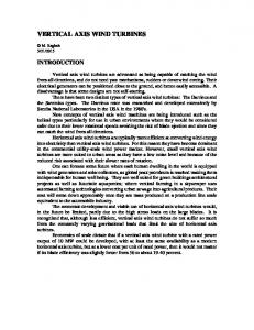
Damping Versus Wind Turbine Rotation Rate Figure 5 shows a plot of modal damping ratio, as calculated with NExT, versus turbine rotation rate for the blade flatwise modes. The plot shows that the damping ratios of these modes generally increase with turbine rotation rate. The increase in damping is quite significant; for example, the first flatwise damping increases from 2 ?6 to 7%. The notable exception is the second blade flatwise mode between 15 rpm and 28 rpm. Such a drop in damping ratio could be due to modal coupling to a more lightly damped mode, since the modal coupling varies with rotation speed. The resulting mode shape could be less affected by the aerodynamic damping terms and, therefore, the damping ratio would drop. Mode shape information is needed to answer this question; however, shape information has not been extracted from this data set. 7

v

1

I

I

I

1

1

6D A N P

I u G

5-

lr

4ma .. .....-..””’”” ,..

2?8 , O\ ‘N,\ ,//0

: T 3$

%

2 */-

/ ./”’ ...““ ....................... ........................74..............””” ./“ 1-------.-.-.-’

0 -o

, 5

1

,

I

1

,

I

10

15

20

25

30

35

40

RPM

Figure

5. Damping of flatwise modes

19

Figure 6 shows a plot of modal damping ratio versus turbine rotation rate for the blade edgewise modes. The trend of increasing damping ratio as rotation rate increases is again seen. The magnitudes of these modal damping ratios are significantly smaller than those of the flatwise modes. Figure 7 shows a plot of the same data for the tower in-plane and tower out-of-plane modes. The damping of the first tower modes have an increasing trend, as seen before. The second tower in-plane mode has an unusual drop in damping ratio at 20 rpm. 2.5

D

I&

2

A M P

I M Q

1.5

R A T ;

1

%

0.5

0 o

5

10

15

20

25

RPM

Figure

20

6. Damping of first and second blade edgewise modes

30

35

40

1.4

1.a

1

0.a

“\ \

0.6

Figure7.

0’

1

1

I

1

1

t

I

-o

5

10

15

20

25

30

35

Damping oftower in-plane andtower

40

out-of-plane males

.

21

Figure 8 contains information about the second and third propeller or rotor twist modes. The notable feature of this plot is the large change in modal damping of the second propeller mode at 10 rpm. The change could be due to coupling with a more highly damped mode. Again, mode shape information will help to clear up this question. 1.1

I

10.9 -

D A M P

0.8 -

I u Q

0.7 -

R A

0.6 -

T :

0.5 0.4 -

% 0.31 0.2 v O.lr 0

, 5

I 10

I 15

1 20

1 25

I 30

1 35

1 40

RPM

Figure

8. Damping of second and third rotor twist modes

Autospectrum

Synthesis

Figure 9 shows a synthesis of the autospectrum of lead-lag strain at the bottom of a 34-m testbed blade while operating at 28 rpm. The synthesis is overlaid on the actual test data. This figure illustrates the usefulness and the limits of this graphical check as well as several aspects of the modal parameter estimation process using NExT. The labels 1P, 2P, 3P, 4P, and 5P denote the per-rev harmonics. The peaks corresponding to the harmonics are seen to be captured well. NExT currently fits the harmonics as though they were actual modes of the system. The first tower in-plane mode, lTi, and the second propeller mode (rotor twist), 2Pr, are a good fit. The near exact synthesis of the position and slope of the peak givesconfidence in the modal frequency and damping ratio from NExT as well as the amplitude coefficient calculated by the autospectrum synthesis. The first blade edgewise mode, lBe, and the second blade flatwise modes, 2F, are seen to have the correct modal frequency estimates, but the autospectrum coefficient was not estimated closely. This could be due to an incomplete mathematical representation of the autospectrum, noise in the experimental autospectrum, or numerical interactions with adjacent modes. The autospectrum synthesis provides little information about the quality of the modal damping ratio estimates in such cases.

22

I

,

I

1

1

1

1

,

I

_l

J

3P&lF SOLID

-

1P DAS~D

T-T

DArA

- nrsrmmm

A

M P L I T v D B

2Pr , 3F&

2P

o

0.5

1

1.5

a

2.5

?REWEJCY

Figure

3

3.5

4

4.5

5

- m

9. Autospectrum and synthesis of lead-lag strain at 28 rpm

The first blade flatwise modes, IF, are coincident with the 3P harmonic. The autospectrum synthesis provides no information about the quality of the modal damping ratio estimate and very little information about the modal frequency estimate in such situations. A technique to estimate and remove the 3P harmonic would probably improve the results. The third blade flatwise modes (3F), the third propeller mode (3Pr), ~d the second tower in-plane mode (2Ti) are closely grouped. Mode shape information is needed to separate these modes. And finally, the second blade egdewise (2Be) is in a region of low signal-to-noise ratio. Information on the fit of this mode should be obtained from different data channels. The comparison of the NExT synthesised autospectrum to the autospectrum of actual operating data shows excellent agreement. However, a few suggestions for improvement can be made. The technique could be improved by providing a method for extracting shape information that could alleviate some problems associated with identifying modes, separating closely spaced modes, or assessing the degree of coupling induced soley by dynamic conditions. Advanced modal analysis techniques [19] are available which could enhance the low amplitude modes, making it easier to estimate their modal parameters.

23

Comparison of NExT Results With Analysis for a Rotating VAWT There are currently two reports that contain analytical predictions of the aeroelastic damping expected during operation of the Sandia/DOE 34-m testbed. Reference 20 reports the work of Lobitz and Ashwill in which the NASTRAN generated damping and stiffness matrices are modified to include the effects of aeroelasticity. Reference 21 includes the work by Malcolm using a modified form of the Lobitz and Ashwill aeroelasticity model. Malcolm’s modifications included terms that model a rotating coordinate frame and an elastic center offset. These references provide the specific information on the assumed analytical models. Figures 10 and 11 compare these analytical results with the damping calculations of NExT. The turbine rotation rate was between 38 and 40 rpm for the data in these comparisons. Figure 10 compares the results for four flatwise modes. The reader is reminded that NExT could not separate the first flatwise modes. However, a clear trend still results, with the predicted damping being higher than the NExT estimates. The damping values are shown as percent of critical viscous damping. Figure 11 compares results for three non-flatwise modes. No clear trend can be seen in these results.

2Fs

1 Fs

1m

2Fa

12, —

I —

10-

—

8—

—

6-

4-

2-

0L

4.

NLM

—

L

NLM

—b.

L

NLM

NLM

N - NExT L - Lobltz and Ashwill M - Malcolm Figure

24

10. Analytical damping results for flatwise modes at 38 rpm

ITI

2Pr

—

—

— —

4.s1

NLM

I

—

NLM

NL

N - NExT L - Iwbltz and Ashwlll M - Malcolm Figure 11. Analytical damping results for non-flatwise modes at 38 rpm

Alternative Applications of NExT NExT is not limited to application on VAWTS. Many structures that are excited in their operating environment such as horizontal-axis wind turbines (HAWTS), offshore platforms, aircraft and aircraft stores, rockets during launch, and ground transportation vehicles may be tested using NExT. An example of the versatility of NExT is provided by a road vibration test recently performed on a tractor-trailer vehicle [22]. The truck was driven 30 miles on an interstate highway at about 55 mph. The data were sampled at 128 Hz and 100 averages were used. Table 3 provides the modal frequencies and modal damping ratios extracted from the data. Performing the modal test using road excitation allowed the nonlinear suspension and tire dynamics to be tested with at-leuel inputs. The capability to test at-level is an important contribution provided by NExT.

25

Table 3. NExT System

Results

Mode 1st Bounce 1st Pitch Tractor Bending 2nd Pitch 1st Trailer Bending Load Mode Trailer Twist Trailer Twist Trailer Twist Trailer Twist

for a Transportation

Frequency(Hz) 1.5 3.2 5.7 6.7 7.0 11.5 15.1 15.7 16.4 17.0

Damping(%) 7.5 1.9 7.6 2.3 3.4 1.1 1.0 1.3 1.1 0.7

Summary A brief overview of NExT has been presented, followed by a theoretical justification. Analytically generated data have been used to verify the ability of NExT to extract modal frequencies and damping ratios from operating data. NExT was further verified by a comparison with conventional modal testing techniques using a parked vertical-axis wind turbine. This same comparison shows the ability of NExT to estimate the total damping of the system. An extra damping mechanism for the flatwise modes of a parked VAWT was implied. This is due to the drag force experienced by a flat plate oscillating parallel to a flowing fluid. Damping versus turbine rotation rate plots have been presented for the DOE/Sandia 34-m testbed over a range of operational rates. A general trend was shown of substantially increasing damping as rotation rate increases. Comparing a synthesized autospectrum with a test data autospectrum is useful for verifying the estimates of the modal parameters. Mode shape information is needed to help explain sudden changes in damping ratio as turbine rotation rate increases, to aid in the identification of higher frequency modes and for verification of autospectrum synthesis coefficients. Advanced modal analysis techniques for extracting information from low-amplitude modes and filtering techniques to remove harmonic peaks are desirable upgrades to NExT. Comparisons between NExT generated results and analytical predictions based on aeroelastic theory illustrate how NExT can be used to provide the necessary information to refine the analytical predictions. The predicted damping of the blade flatwise modes was higher than the damping estimates provided by NExT. However, no clear difference was seen in the predicted damping for the non-flatwise modes. The inability of NExT to separate the first blade symmetric and antisymmetric modes indicates the need to develop techniques to separate closely spaced modes. Several alternative applications for NExT have been suggested. An example of the versatility of NExT using a tractor-trailer vehicle excited by road irregularities experienced at highway speeds was presented. The modal frequencies and damping ratios extracted from this operational test are representative of the at-level response the truck will see in service.

26

APPENDIX

A

Frequency Shifts in VAWT-SDS

Code

In assessing our ability to estimate modal frequencies and damping from transient response data, we had occasion to use Dohrmann’s VAWT-SDS Code to generate time responses. Since this was a simulation exercise, the “exact” modal frequencies and damping were available from the eigenvalues obtained from the finite-element representation of the mass, stiffness, and darnping matrices. We discovered that our estimated modal frequencies were proportionally lower than the known exact values. This phenomenon was found to be caused by the numerical integration process. These effects are discussed by Bathe and Wilson [14]. A method to calculate frequency and amplitude changes in frequency response functions resulting from numerical integration was provided by Rodeman [23]. We have recently expanded on this work to allow direct calculations of the changes in modal frequency and modal damping ratio. The derivation of this technique is provided. The Newmark integration scheme is driven by the following equations: ut+T

ut+T —

Ut

. — Ut =

=

[(l–a)ut+ fiit+T] T

utT +

(A-1)

[(:-a)ut+aut+dT2 (A-2)

where a and 6 are integration parameters, and T is the sampling interval. The differential equation for the mode of interest is: ..

ut=ft

—2fuut

.

—u2ut

(A-3)

where u is the undamped natural frequency ~ is the damping ratio f is the applied force. Take the z transform of Equations (l), (2), and (3): (z–l)U

(z–l)U

= T[z6 + (1–6)]U

= TU + T’

[az+b)lu

U= F–2(’UU-U2U

(A-4)

(A-5)

(A-6)

where capital letters denote transformed variables.

27

From Equation (4): ~ =

[(T6)z + T(l–@l (z–1) {

~

(A-7)

“

1

Now, substituting Equation (7) into Equation (5):

(z–1)

u=

[(T20z + T’(l–rS)] (z–1) {

‘[(T2a)z+T2(Hlu (A-8)

Substituting Equation (7) into Equation (6): U=F–

[(2r@Ta)z +(2r@T)(l–a)l (z–1) (

~_@2u

(A-9)

)

Solving Equation (9) for U: ..

(z–l)

(F–u2U)

u = [(2J~ T6+1) Z + (2roT–2taT6

– 1)] “

(A-1O)

Substituting Equation (10) into Equation (8) and solving for U:

where

u= blz a1z2+a2z+a3 T2F ( 2 + b2z + b3)

(A-n)

al=a 1 a2=~+8—2a 1 a3=j+6+a bl = Q 2T 2al + 2f_uT6+ 1 b2 = a2T2a2 + 2f~T(l – 26) – 2 b~ = o. 2T2as – 2ftiT(l–

6) + 1.

Now let Z1 and z1* be the complex conjugate solutions of the denominator .polynomial: bl(zl) 2 + b2 (z1) + b3 = 0.

(A-12)

ZI is then the discrete eigenvalue for the system. It must be converted to a continuous eigenvalue sl:

28

zl = ~SIT

(A-13)

Z1 = Zr + iZi

(A-14)

al = Sr+ iSi

(A-15)

i= sl =:10 ~

(A-16)

ge G% +

Sr=Lo ~T

Si=—

J1—

ge

tzr2

;h–l

@

+

%9

q .

() Zr

(A-17)

(A-18)

(A-19)

Assuming light damping, the shifted values are given by the following: U* = Si

(A-20)

(A-21)

If we specialize the above results to the unconditionally stable Newmark-@ scheme we have that

1 a =-4 Now, if we further examine the effects of this integration scheme on an undamped mode, the coefficients in Equation (12) specialize to 2

bl=l+$

bz=2

() [() 1

b~=l+~

uT2’ ~ –1

UT 2

(A-22)

.

()

29

Then the roots associated with Equation (12) are given explicitly as

‘=[(a2-1*’uTl[1 +F)21-1

(A-23)

Upon substituting Equation (23) into Equation (18) we get s, = O, which implies that the mode is also undamped after integration. This is in agreement with the fact that this specific integration scheme is unconditionally stable. From Equations (19) and (23) in conjunction with (20), we obtain 1

U* = ---tan-l

~T

[01 2“

(A-24)

1– :

Note that for UT small, Q* = O, that is the natural frequency after integration is equal to the natural frequency, before integration. For a specific time step and natural frequency Equation (24) provides an explicit expression where the classic period elongation associated with the Newmark-D can be determined. Table A-1 provides the results of this work. The data presented in this table were generated by the VAWT-SDS code. The unconditionally stable Newmark-fl algorithm (a = 0.25, 6 = 0.5) with a step size of 0.04 second was used for integration. The table provides the frequency and damping values that were specified for each mode. These values were calculated by extracting the mass, damping, and stiffness matrices from the VAWT- SDS code and solving the appropriate eigenvalue problem. A static condensation [24] was performed to remove all degrees of freedom with zero inertia terms. Then an undamped eigenvalue problem was solved. The first 300 eigenvectors were used to further reduce the damped eigenvalue problem [25]. It should be noted that these frequencies closely match previously reported solutions of the undamped problem. Figure 9.3 of .Reference 14 provides the information necessary to correct the frequencies for the numerical integration. These corrected frequencies are included in Table A-1 as well as the corrected modal frequencies and corrected modal damping values generated by our algorithm given above. The close correspondence between the values calculated from information provided by Reference 14 and those calculated from the algorithm provides confidence in the algorithm. The modal frequencies and modal damping ratios as calculated by NExT and reported in Table 1 are repeated in Table A-1. The close correspondence between the NExT results and the corrected frequencies shows that frequency shifting was indeed occurring.

a

*

30

Table

A-l.

Effect

of Frequency

Shift Corrections

on Simulated

Results

Specified Specified Corrected* Corrected3 Corrected3 Calculated’ Calculated Fre~~uncy Dammp~ Fr ~ u:~y Fr~;umy Dammp~ Fr~;;ncy D~%p~ % Mode lPr lFa IFs lB lTi 2Fs 2Fa lTo 2Pr 2Ti 3Fa 3Fs 3Pr 2B

0.228 1.28 1.36 1.61 2.06 2.51 2.59 2.92 3.61 3.69 3.93 4.03 4.04 4.22

4.72 0.19 0.20 0.26 0.32 0.40 0.37 0.34 0.58 0.57 0.57 0.69 1.14 0.58

0.228 1.27 1.35 1.59 2.02 2.44 2.51 2.79 3.39 3.46 3.64 3.72 3.73 3.85

0.228 1.27 L35 1.59 2.02 2.43 2.50 2.80 3.39 3.46 3.65 3.73 3.74 3.88

4.72 0.19 0.20 0.25 0.31 0.38 0.35 0.31 0.51 0.50 0.49 0.59 0.98 0.49

1.31 1.32 1.59 2.01 2.44 2.50 2.80 3.39 3.46 3.63 3.73

0.35 0.34 0.29 0.38 0.50 0.38 0.52 0.59 0.44 0.36 0.38

3.87

0.34

1 Determinedby Eigenanalysis. 2 CorrectedusingReference14 in mainreport. 3 Correctedusingalgorithmfrom AppendixA. 4 CalculatedusingNExT.

31-32

APPENDIX

B

Calculation for Drag Damping on a Vibrating Flat Plate Figure B-1 shows the model for this analysis. This is a single degree-of-freedom system, but it can be used to illustrate the damping mechanism observed on the turbine blade. The mass, m, stiffness, k, and darnping, c, represent the modal mass, modal stiffness, and modal damping of a FloWind 19-m VAWT blade oscillating in the first blade flatwise mode. The physical motion of the blade is represented by u(t). For a blade this motion would actually be a function of the distance along the blade. However, for these calculations, it will be assumed that the displacement is uniform. The mean wind velocity and direction is denoted by VO and assumed to be steady.

V.

k

u(t)

c Figure

B-1.

Oscillating flat plate which is normal to a wind

The equation of motion for this representative single degree-of-freedom system is given by mu(t) + cu(t) + ku(t) = F(t) where F(t) is the external forcing function caused by the interaction of the plate with the wind. This forcing function is fiven below [18]: F(t) = C~A ~ pV 2 sgn(V) where Cd is the effective coefficient of drag of the turbine blade; A is the effective area of the blade that is normal to the wind direction; and sgn(V) is the sign of V. The blade is assumed to be oriented flatwise to the wind. The mass density of the air is given by p. The total relative velocity of the blade and the air is: v(t) = v~ – u(t).

33

The following magnitude approximations are used in this analysis:

V(I-

22mphandlul