The least squares fit reciprocal modal vector is determined for a set of experimental FRFs. The correlation coefficient is used to determine the quality of fit. This is ...
A MODAL PARAMETER EXTRACTION ALGORITHM USING BEST-FIT RECIPROCAL VECTORS David D. Johansen Mechanical Engineering Department Michigan Technological University Houghton, Ml 49931
Randall L. Mayes Experimental Structural Dynamics Department Sandia National Laboratories Albuquerque, NM 87185
ABSTRACT
The dot product of a reciprocal modal vector with a vector of frequency response functions (FRFs) can produce a generalized coordinate FRF that has single-degree-offreedom response. A modal extraction algorithm is developed based on this concept. A generalized coordinate FRF is assumed with a corresponding frequency and damping. The least squares fit reciprocal modal vector is determined for a set of experimental FRFs. The correlation coefficient is used to determine the quality of fit. This is done for several discrete frequency and damping values that cover the parameter space of interest. Over this parameter space, local maxima of the correlation coefficient can be used to identify roots of the system. An example is given utilizing experimental data.
NOMENCLATURE
FRF: frequency response function SDOF: single-degree-of-freedom natural frequency of r'th mode w,: damping coefficient of r'th mode 1;;,:
: '1': Hp(w): A,: j:
mode shape matrix reciprocal modal (weighting) vector analytical generalized coordinate FRF modal residue coefficient
influenced by the locations of exciters and sensors, the estimation algorithm used, the frequency band utilized and the model order assumed. Estimation is further complicated if the frequencies are closely spaced and the damping ratios of some or all of these roots is high. Uncertainty in closely spaced roots amplifies the uncertainty in the associated mode shapes which can lead to wrong understanding of the structural dynamics. When absolute response predictions are desired, a particular concern is the uncertainty in damping coefficient estimates, which are highly susceptible to errors 111 • Much effort has been focused on reducing uncertainties, both experimentally and mathematically. Multiple averages reduce uncorrelated noise. Optimal test design algorithms increase the likelihood of strongly exciting and observing modes of interest. Proper combination of input signal selection and data windowing can decrease the uncertainty associated with damping. Once the data has been obtained, a variety of different mathematical methods can be employed to identify the true underlying signal. Least-squares methods are used to minimize the squared error between the model Principal Components Analysis and experimental data. (PCA) utilizes the Singular Value Decomposition (SVD) to eliminate noise, providing a means of favorably weighting the data to improve matrix conditioning. To reduce uncertainty in frequency and damping, a new type of estimation algorithm has been developed. This approach, termed the "Synthesize Modes And Correlate" (SMAC) 121 algorithm, is based on the principles of modal filtering •
r-1
Introduction And Motivation
Theory
Experimental roots (natural frequencies and damping ratios) of a system are determined through the process of parameter estimation. As the process name implies, there is a level of uncertainty in the results obtained. Variations are
During the last two decades, modal filtering 12-51 has been investigated in regards to control and reducing uncertainty. A modal filter is a matrix of weighting vectors, sometimes called reciprocal modal vectors, that transforms physical coordinates into modal coordinates. Each reciprocal modal vector transforms the physical coordinates into one associated modal coordinate. The concept is extended to FRFs in the following way. Beginning with the modal substitution,
This work was performed at Sandia National Laboratories and supported by the U.S. Department of Energy under contract DE-AC04-94AL85000.
517
[ ]{p} = {x}
(1)
where p is the vector of generalized coordinates, is the mode shape matrix and x is the vector of physical coordinates. To obtain the generalized coordinates alone, (2) and then transposing, (3)
If we define
{'¥}
of the columns of
as the reciprocal modal vector that is one
[
rr '
ro, is the modal frequency, roi is the frequency at line j, 1;, is the viscous damping ratio, A, is the residue coefficient for the mode under consideration and
'¥;
is a scalar.
In traditional modal filtering both the experimental response and weighting vector are known, leaving the uncoupled response to be solved for. The proposed technique requires knowledge only of the experimental data and synthesis of an assumed analytical FRF (here the assumption is based on real modes). By assuming a natural frequency and damping coefficient, an analytical SDOF accelerance FRF is created in the above form. The residue coefficient has been arbitrarily set to unity. This FRF is multiplied by the pseudoinverse of the experimental data to create a least-squares weighting vector, i.e. the calculated reciprocal modal vector, or mathematically
transform into the frequency
domain and divide by a single input force, then
(6) (4)
where {Hp} is a SDOF FRF, [Hxl is a set of FRFs from a single input, and
{'¥}
experimental
is the reciprocal modal
vector. The matrices in equation (4) are expanded as
-A ' a/I m~+ j2(,m,m 1 -W~
-A '
If the assumed modal frequency is a mode of the system, the weighting vector will be orthogonal to all modes except for the one of interest, and a single-degree-of-freedom (SDOF) FRF can be reconstructed with the weighted sum of the experimental FRFs (see the first plot of Figure 1). However, if the assumed modal frequency is not a mode of the system, the weighted sum will provide a poor reconstruction of the analytical SDOF FRF (see the second plot in Figure 1). 20,----.----.----.----r----r----.---~----.
W
2 2
15
ffltural
frequency:~:
75.9 Hz
Da~Tplng
=2.6%
10-
oL~---~/~--~==~==-==~==~~~-~-~~---~-=--=-~-=·~·-=--~-0 50 100 150 200 250 300 350 400
2 m,2+ 1"21' '=' ,m,mNs-mNs
Hl(wl)
H, (wJ
[HJ= ~JmJ
H, (m,)
{'¥}=
Frequency (Hz)
Figure 1 - Comparison of A Good and Poor Reconstruction With the Assumed Frequency and Damping (Smooth line is analytical SDOF FRF and jagged line is weighted sum of experimental FRFs)
(5)
NS is the number of spectral lines, NO is the number of output locations in the experimental accelerance FRF matrix,
Performance of the reconstruction attempts is measuring the correlation coefficientr•> between FRF and the weighted sum of experimental correlation is focused on the region around
518
monitored by the analytical FRFs. This the peak to
enhance identification of the damping coefficient, because the strongest effects of damping are seen near resonance. If the correlation coefficient between these two FRFs is 1, then the assumed natural frequency and damping are taken to be a root of the system. This is an iterative approach, where after one pair of frequency and damping values is evaluated, a new pair is assumed until the entire ranges of interest in both frequency and damping have been analyzed (Figure 2}. Notice that the indication of modes along the frequency axis is strong, while the indication of modes along the damping axis is much less precise. This is consistent with the community experience that it is easier to identify the frequency accurately than the damping.
Correlation Coefficient with 2% Damping
r
\ 0.9 0.8 0.7
y
I~
~ J
0.6
~-0.5 8 0.4 0.3
~
0.2 0. 1
0 o
20
40
60
ao
100
120
140
160
1ao
200
FreQuency
Figure 3 - SMAC Correlation Coefficient Plot
0.8
In Figure (4) the Normal Mode Indicator Function for the data is compared with the correlation coefficient. It can be seen that several modes not observable or weakly observable in the Normal Mode Indicator Function were indicated in the SMAC plot. 0.05
Frequency {Hz)
12°oatA>ing coefficient
Figure 2 - 30 Plot of Correlation Coefficient Implementation
This algorithm was developed using an experimental set of FRFs that contained many highly damped and closely spaced modes. The algorithm was implemented with an assumption of real modes, i.e. the residue for HP in equation (5} is a real number. The solution of equation (6} was constrained to obtain real valued weights to decrease the solution time. An initial damping ratio was assumed. Then equation (6} was solved at every frequency line of the experimental data. (It is not required that every frequency line be utilized. By the same token, the solution could be found between the experimental frequency lines, but we chose to utilize the experimental frequency lines.} Then the correlation coefficient for the vectors from each side of equation (4} were calculated at each experimental frequency line. This was plotted, and the peaks were indications of modes (see Figure 3}.
519
v
v
~(~
1\ (\ 1\ ~ (\
I VJ v
O,BOO(I
vv
v
0,401)(1
.
'00
P r • 'I u • n c
'
.\11
1:1J4~"'Y•2
r
Correlation Coefficient with 2% Damp1ng
\ 0.9
0.8 0. 7
D. 6
~
J
~
~0. 5 0
0. 4 0. 3
~
0. 2 0. 1
20
If the spatial independence of the mode shape cannot be defined well by the accelerometers, it has been observed that such modes do not have as strong an indication of the mode using the SMAC algorithms. It has also been observed that in frequency bands where the signal to noise ratio is low, SMAC may give high correlation coefficients, even where there are no true modes (see the very low frequency band in Figure 3}. However, SMAC algorithms seem to be very robust at detecting weakly excited modes and closely spaced modes with fairly high damping ratios, on the order of two to five percent. SMAC has detected some modes with three to five percent damping that have not been able to be extracted with the Direct Parameter Estimation or Polyreference Time Domain methods. Future Work
~
0
minimum error that was truly there. This can be understood by observing Figure 2 in the damping axis. The correlation coefficient surface gets very flat with higher damping values. For true roots, it has been found that there is usually a peak, but by choosing the damping bounds to be too wide, the local maximum can be missed.
40
60
80
100
120
140
160
180
200
Frequency
Figure 4 - Comparison of the Normal Mode Indicator Function with the SMAC Correlation Coefficient At this point, the user could select a narrow bandwidth about any peak of interest and perform an optimized search for the root in a smaller domain. Two optimization methods have been programmed in MATLAB. One is called the golden section search 1"1• This algorithm attempts to find a local maximum of the correlation coefficient in the region the user specifies for frequency and damping. It was found that the maximum in correlation coefficient was more distinct if only a few frequency lines on either side of the assumed analytical frequency were utilized in the correlation coefficient calculation. It was found that five to ten lines on each side of the assumed frequency worked well for this data set. The second method utilized a constrained optimization routine in MATLAB191 (the "constr'' command in the optimization toolbox). This optimization routine attempts to minimize the squared error between vectors on either side of equation (4). Upper and lower bounds were specified by the user. It was found that if too large a range of damping bounds was investigated, the algorithm might not find the
The modal extraction approach presented has shown promise in improving the estimates of modal frequencies, and particularly damping. However, as stated above, this algorithm has assumed real modes. The effects of complex modes (particularly phase shifts) on the correlation coefficient need to be investigated and accounted for. Additionally, the matrix manipulations in the algorithm were formulated for data obtained from a single excitation location. To identify repeated roots, FRFs obtained from multiple input locations are required 171 • It is thus necessary to design a multiple input format to identify repeated roots, which involves determining the participation factors of each mode. Finally, this algorithm needs to be intensively examined to quantify its advantages and disadvantages. These topics will be presented in a future paper. Conclusions The SMAC algorithm appears extremely robust in extracting weakly excited modes from test data. Therefore, the modes are less likely to go undetected, even if they are highly damped. A second advantage is that the algorithm is valuable in isolating closely spaced roots. Since its calculations can be made for frequencies between adjacent frequency lines of the FRFs, it is not limited to the resolution of the FRF measurement. SMAC definitely indicates modes that other mode indicator functions may not detect. A disadvantage is that it is not easy to distinguish excited modes from weakly excited modes with correlation coefficient as it is now implemented. For reason, it is of value to use SMAC in conjunction
520
well the this with
accepted mode indicator functions to separate well excited modes from weakly excited ones.
[9] Grace, Andrew, Optimization Toolbox For Use With MATLAB, The Mathworks, Inc., 1992, pp2-22.
The technique seems to work better for determining roots for moderately damped modes than some commercial algorithms. However, plots of the correlation coefficient vs damping show that it becomes more difficult to determine the true value of the damping as the damping ratio becomes large. The algorithm assumes real modes, and is robust in determining the roots if the modes are approximately real. If the modes are too complex, it is not known whether the current formulation is sufficient. Theoretically, SMAC can detect the existence of two modes at exactly the same frequency with different damping ratios, but this capability has not yet been proven in practice. Since the algorithm is based on the modal filter, a reasonable test design is required so that the number and placement of sensors is adequate to determine a reciprocal modal vector that will produce a SDOF response when multiplied by the FRF vector. References
[1] Ibrahim, S.R., "Double Least Squares Approach for Use in Structural Modal Identification", AIAA Journal, vol. 24(3), pp499-503, March 1986. [2] Johansen, D.O., "The Development and Evaluation of a New Modal Identification Algorithm Based on the Theory of Modal Filtering", Master of Science Thesis, Department of Mechanical Engineering, Michigan Technological University, 1997. [3] Shelley, S.J. and Allemang, R.J., "Calculation of Discrete Modal Filters Using the Modified Reciprocal Modal Vector Method", Proceedings of the 1dh /MAC, pp37-45, 1992. [4] Zhang, Q., Allemang, R.J. and Brown, O.L., "Modal Filter: Concept and Applications", Proceedings of the Efh /MAC, pp487-496, 1990. [5] Mayes, R.L. and Carne, T.G., "Extraction of Modal Parameters with the Aid of Predicted Analytical Mode Shapes", Proceedings of the 14'h /MAC, pp267 -272, 1996. [6] Thomas, L.F. and Young, J.l., An Introduction to Educational Statistics: The Essential Elements, Third Edition, pp77, 1993. [7] Void, H., Kundrat, J., Rocklin, G.J. and Russell, R., "A Multi-Input Modal Estimation Algorithm tor MiniComputers", SAE Paper#B20194, pp815-821, 1983. [8] Gill, Phillip E., Murray, Walter and Wright, Margaret H., Practical Optimization, Academic Press, San Diego, California, 1981, pp90-91.
521