Life-cycle cost assessment of mid and high-rise steel and reinforced concrete-composite minimum building cost designs Nikos D. Lagaros1 and Efrossini Magoula Institute of Structural Analysis & Seismic Research, National Technical University Athens Zografou Campus, Athens 157 80, Greece E-mail:
[email protected],
[email protected]
Abstract: The traditional trial-and-error design approach is inefficient to determine an economical design satisfying also the safety criteria. Structural design optimization, on the other hand, provides a numerical procedure that can replace the traditional design approach with an automated one. The objective of this work is to propose a performance-based seismic design procedure, formulated as a structural design optimization problem, for designing steel and steel-concrete composite buildings subject to interstorey drift limitations. For this purpose eight test examples are considered, in particular four steel and four steel-concrete composite buildings are optimally designed with minimum initial cost. Life-cycle cost analysis (LCCA) is considered as a reliable tool for measuring the damage cost due to future earthquakes that will occur during the design life of a structure. In this study LCCA is employed for assessing the optimum designs obtained for steel and steel-concrete composite design practices. Keywords: Performance-based design; fibre modelling; steel and steel-reinforced concrete composite buildings; multicomponent incremental dynamic analysis; life-cycle cost analysis; particle swarm optimization
1
Corresponding author
1
1.
INTRODUCTION
The modern conceptual approach to structural design under seismic loading is based on the principal that a structure should meet performance objectives for a number of hazard levels, ranging from earthquakes of small intensity with small return period, to more destructive events with large return period. This approach constitutes the performance-based design (PBD) concept which has been introduced in order to increase the safety against natural hazards. According to PBD the structures should be able to resist earthquakes in a quantifiable manner and to present levels of desired possible damage. The current state of practice in performance-based engineering can be found in US guidelines such as ASCE-41 (2006), FEMA445 (2006) and ATC-58 (2009). Towards this goal, these guidelines suggest higher-order analysis procedures for the design and assessment in seismic prone areas. A highly-efficient design framework can be offered by structural optimisation taking advantage of the benefits offered by nonlinear, static or dynamic analysis methods. PBD formulated as a structural optimisation problem is a topic of growing interest and has been the subject of extensive research over the last years. Advancements in structural optimisation have made possible the move from traditional trial-and-error design procedures towards fully automated approaches based on a structural optimisation search-engine. This is mostly attributed to the rapid development of metaheuristic optimization methods, which are capable of handling complicated structural problems. In construction industry decision making for structural systems situated in seismically active regions, requires consideration of damage cost and other losses resulting from earthquakes occurring during the lifespan of a structure. Nowadays life-cycle cost analysis (LCCA) becomes an essential component of the design process used to control the initial and the future cost of building ownership. In early 1960s LCCA was applied in the commercial area and in particular in the design of products considering the total cost of developing, producing, using and retiring. The introduction of LCCA in construction industry was made in the field of infrastructures as an investment assessment tool. In particular, in early 1980s it was used in USA as an appraisal tool for the total cost of ownership over the lifespan of an asset (Arditi and Messiha, 1996; Asiedu and Gu, 1998). Later, in view of large losses due to extreme hazards, like earthquakes and hurricanes, there was a need for new design procedures of facilities that could lead to life protection and reduction of damage and economic impact of such hazards to an acceptable level (Wen and Kang, 2001b). In this context LCCA was introduced in the field of constructions as an investment appraisal tool incorporating a structural performance criterion (Sanchez-Silva and Rackwitz, 2004). 2
In recent years, steel-reinforced concrete composite buildings have been experiencing increasing applications worldwide. This is because reinforced concrete (RC) is not expensive and RC members are stiff; on the other hand steel members are strong, lightweight and easy to assemble. In composite columns two systems are commonly used: (i) steel reinforced concrete members, where a steel section is encased in concrete and (ii) concrete filled tubes. In many cases, the choice of either of the two systems is based on their excellent resistance to seismic loading. The objective of this work is the formulation of a performance-based optimum design framework for designing steel and steel-RC composite moment resisting building structures subject to interstorey drift limitations with reference to their initial cost considering various types of design practices (steel or steel-RC composite and with or without bracings) in order to study their influence on the resulted design. For this purpose mid and high-rise steel and steel-RC composite 3D buildings are considered, while LCCA is performed for assessing the optimum designs obtained. In particular steel-RC composite buildings build of steel sections encased in concrete are considered, while design practices with and without bracings are also taken into account.
2.
LITERATURE SURVEY ON PBD OPTIMIZATION
A number of studies have been published in the past where the concept of performance-based design optimization was studied. Among others, Fuyama et al. (1994) presented a computerbased design methodology for the control of interstorey drift caused by equivalent static earthquake loads in tall moment resisting steel frame structures. Beck et al. (1999) presented a general framework for multi-criteria optimal design which is well suited for performancebased design of structural systems operating in an uncertain dynamic environment. Ganzerli et al. (2000) proposed a performance-based optimization procedure of reinforced concrete (RC) frames using a mathematical optimizer. Esteva et al. (2002) presented a life-cycle formulation for the determination of optimum values of the mechanical properties of a structural system exposed to seismic risk. The resulting values were used for the establishment of performanceacceptance criteria for seismic design. Khajehpour and Grierson (2003) investigated the tradeoff between life-cycle profitability and load-path safety for a high-rise office building project, while they proposed alternative building layouts with increased safety using a multi-criterion genetic algorithm (GA). Li and Cheng (2003) introduced a damage reduction based technique in the framework of structural optimization and showed that the proposed design concept leads to designs with better seismic performance in terms of both life-cycle cost and maximum interstorey drift criteria. Chan and Zou (2004) presented an effective optimization technique for the elastic and inelastic drift performance design of reinforced concrete buildings 3
under response spectrum loading and pushover loading. Liu et al. (2005) proposed a GAbased multi-objective structural optimization procedure for steel frames considering four objective functions; weight, maximum interstorey drift for two performance levels, and design complexity criteria. Chan and Wang (2005) developed an optimality criteria based algorithm for solving the minimum weight design problem subject to multiple drift constraints and member sizing requirements. Fragiadakis et al. (2006a) proposed a performance-based optimization procedure for steel moment-resisting frames in the probabilistic framework of FEMA-350 (2000). Fragiadakis et al. (2006b) proposed a new methodology for the performance-based optimum design of steel structures subjected to seismic loading considering inelastic behaviour, while the importance of considering life-cycle cost as an additional objective to the initial structural cost objective function in the context of multi-objective optimization was also investigated. Foley et al. (2007) presented an overview of a state-of-the-art modelcode performance-based design methodology and implemented this design procedure into multiple-objective optimization problems for single and multi-storey structural steel frameworks with fully and partially restrained connections. Lagaros and Papadrakakis (2007) evaluated the European seismic design code when used for the design of 3D reinforced concrete buildings, versus a PBD procedure, in the framework of a multi-objective optimization concept. Rojas et al. (2007) used GA to solve this complex optimization problem where confidence levels were incorporated into the fitness function along with initial construction cost in a series of optimal design scenarios. A fully automated design methodology based on nonlinear response history analysis was proposed by Fragiadakis and Papadrakakis (2008b) for the optimum seismic design of reinforced concrete structures. Lagaros et al. (2010) proposed a PBD methodology for the design of reinforced concrete buildings, taking into account the influence of infill walls, while two variants of the PBD framework are examined relying either on the non-linear static or on the non-linear dynamic analysis procedure. Kaveh et al. (2010) presented a performance-based optimal seismic design of frame structures using the ant colony optimization method. The current state-of-practice static pushover methods as suggested in the provisions of European and American regulations are implemented in a comparative study by Lagaros and Fragiadakis (2011), in a performance-based design optimization framework. Esteva et al. (2011) presented an overview of life-cycle optimisation in the establishment of reliability and performance-based seismic design requirements for multi-storey systems. AlAnsari and Senouci (2011) presented a drift design structural model for the design optimization of high-rise buildings in seismic zones. Fragiadakis and Lagaros (2011) presented a general PBD optimization framework for steel structures; while in Mitropoulou et al. (2011)
4
presented a multiobjective life-cycle optimisation problem examining the parameters that affect the LCCA procedure.
3.
PERFORMANCE-BASED SEISMIC DESIGN
The majority of the seismic design codes belong to the category of the prescriptive design codes, which take into consideration site selection and development of the conceptual, preliminary and final design stages. According to a prescriptive design code the strength of the structure is evaluated at one limit state, between life-safety and near collapse, using a response spectrum-based loading corresponding to one or two design earthquakes (e.g. Eurocode 8, 2004). In addition, the serviceability limit state is usually checked in order to ensure that the structure will not deflect or vibrate excessively. On the other hand, performancebased design implies the design, evaluation, construction and maintenance of engineering facilities in order to meet the objectives set by the society and owners/users of a facility (Krawinkler and Miranda, 2004). In the case of earthquakes, the aim is to build structures having a predictable and reliable performance, or in other words, to be able to resist earthquakes with quantifiable confidence. Therefore, the modern conceptual approach of seismic structural design is that the structures should meet performance-based objectives for a number of different hazard levels ranging from earthquakes with a small intensity and with a small return period, to more destructive events with large return periods. The current state of practice in performance-based earthquake engineering is defined by US guidelines (ASCE-41, 2006; FEMA-445, 1996; ATC-58, 2009). These guidelines do not differ conceptually and introduce procedures that can be considered as the first significant diversification from prescriptive building design codes. Many of the current codes for the design of new buildings are only partially performance-based, since they attempt to tie all design criteria to one performance level, usually to that of life safety or collapse prevention. The main part in a performance-based seismic design procedure is the definition of the performance objectives. A performance objective is defined as a given level of performance for a specific hazard level (see Figure 1). In order to assess the structural performance in terms of strength and deformation capacity globally as well as at the element level a nonlinear analysis procedure is required. In this work the PBD framework is based on the nonlinear static procedure (NSP) where the structural model is “pushed” according to a predefined lateral load pattern. In order to determine the target displacement in multiple hazard levels required by the performance-based design framework, typically one of the following methods is adopted: the capacity spectrum method of ATC-40 (1996), the coefficient method of ASCE-41 (2006) and the N2 method of EC8 (2004). According to ASCE-41, apart from a first-mode based lateral 5
load pattern the use of a uniform pattern is also suggested. In the numerical results that follow only the first-mode pattern was taken into consideration. For 3D structures the properties of the lateral load pattern have to be extracted from the mode that refers to the direction under consideration. According to ASCE-41 (2006) the target displacement, which is the displacement of a characteristic node on the top of a structure during a given seismic event, typically in the roof, is defined with the aid of the formula
dt C0C1C2C3 S a
Te2 g 4 2
(1)
where C0, C1, C2 and C3 are modification factors, discussed in the FEMA-440 (2005) guidelines and Te is the effective fundamental period of the building.
4.
LOWER BOUND STRUCTURAL DESIGN
The ultimate objective of this study is to compare lower-bound designs, or in other words comparing the designs that satisfy design requirements in the most cost-effective way, i.e. those with minimum cross section dimensions, member and reinforcement steel quantities. For this reason, a structural optimization problem is formulated and the designs obtained are then assessed. The formulation of a structural optimization problem is defined as follows
min sF
CIN (t , s )
subject to g SERV (s) 0 j =1,...,m j
(2)
g PBD (s) 0 j =1,...,k j where s represents the design vector with the cross-section dimensions of all columns and beams, F is the feasible region where all the serviceability and performance-based constraint functions (gSERV and gPB) are satisfied, while the objective function considered is the initial cost CIN of the design, which is related to material cost, which includes structural steel, concrete, steel reinforcement, construction labour costs and the cost of the non-structural elements. Additionally, the cost of the contents is included. The performance-based constraints considered are related to the maximum interstorey drift limits θ. This is a commonly used measure of both structural and non-structural damage because of its close relationship to plastic rotation demands on individual beam-column connection assemblies. In this study three performance objectives are considered corresponding to hazard levels of 50, 10 and 2 percent probabilities of exceedance in 50 years. The detailed description of the exact steps followed for the seismic design of the buildings can be found in the work by Lagaros and Papadrakakis
6
(2007), while a flowchart of these steps is presented in Figure 2, where a nonlinear static analysis method is nested in the iterative optimum design algorithm. For the solution of the optimization problem the particle swarm optimization method (PSO), is employed. In particle swarm optimization (Kennedy and Eberhart, 1995), multiple candidate solutions coexist and collaborate simultaneously. Each solution is called “a particle” having a position and a velocity in the multidimensional design space while a population of particles is called a swarm. A particle “flies” in the problem search space looking for the optimal position. As “time” passes, a particle adjusts its velocity and position according to its own “experience” as well as the experience of other (neighbouring) particles. A particle's experience is built by tracking and memorizing the best position encountered. PSO combines local search (through self-experience) with global search (through neighbouring experience), attempting to balance exploration and exploitation. Each particle maintains its two basic characteristics, velocity and position, in the multi-dimensional search space that are updated as follows
v j (t 1) wv j (t ) c1r1
s Pb,j s j (t ) c2r2 s Gb s j (t )
s j (t 1) s j (t ) v j (t 1)
(3) (4)
where vj(t) denotes the velocity vector of particle j at time t, sj(t) represents the position vector of particle j at time t, vector sPb,j is the personal best ever position of the jth particle, and vector sGb is the global best location found by the entire swarm. The acceleration coefficients c1 and c2 indicate the degree of confidence in the best solution found by the individual particle (c1 cognitive parameter) and by the whole swarm (c2 - social parameter), respectively, while r1 and r2 are two random vectors uniformly distributed in the interval [0,1]. The symbol “ ” of Eq. (3) denotes the Hadamard product, i.e. the element-wise vector or matrix multiplication. Figure 3 shows the flowchart of the PSO algorithm, while Figure 4 depicts a particle’s movement in a two-dimensional design space. The particle’s current position sj(t) at time t is represented by the dotted circle at the lower left quadrant of the drawing, while the new position sj(t+1) at time t+1 is represented by the dotted bold circle at the upper right hand of the drawing. Figure 4 depicts how the particle’s movement is affected by: (i) it’s velocity vj(t); (ii) the personal best ever position of the particle, sPb,j, and (iii) the global best location found by the entire swarm, sGb.
7
5.
LIFE-CYCLE COST ANALYSIS OF STRUCTURES
The total cost CTOT of a structure, may refer either to the design-life period of a new structure or to the remaining life period of an existing or retrofitted structure. This cost can be expressed as a function of the time and the design vector as follows (Wen and Kang, 2001a)
CTOT (t , s) CIN ( s) CLS (t, s)
(5)
where CIN is the initial cost of a new or retrofitted structure, CLS is the present value of the limit state (or life-cycle) cost; s is the design vector corresponding to the design loads, resistance and material properties, while t is the time period. The term “initial cost” refers to the cost of a new structure for the construction or to the money invested on an old structure for its retrofit. The term “limit state cost” in this work refers to the potential damage cost from earthquakes that may occur during the life of the structure. It accounts for the cost of the repairs after an earthquake, the cost of loss of contents, the cost of injury recovery or human fatality and other direct or indirect economic losses related to loss of contents, rental and income. Damage may be quantified by using several damage indices (DIs) whose values can be related to particular structural damage states. So far a large number of researchers have studied various damage indices, while a detailed survey can be found in the work by Ghobarah et al. (1999). Damage, in the context of life cycle cost analysis, means not only structural damage but also non-structural damage. In this work the maximum interstorey drift (θ) has been considered as the response parameter which best characterizes the structural damage, associated with all types of losses. The relation between the drift ratio limits with the damage states, employed in this study (Table 1), is based on HAZUS (2003). On the other hand, the response quantities associated with the loss of contents like furniture and equipment is the maximum response floor acceleration. The relation of the limit states with the values of the floor acceleration used in this work (Table 1) is based on the work of Elenas and Meskouris (2001). The limit state cost (CLS) for the ith limit state can be expressed as follows i , i i , i i CLS Cdam Ccon Cren Cinc Cinji C ifat
(6a)
i ,a i ,a CLS Ccon
(6b)
i i , where Cdam is the damage repair cost, Ccon is the loss of contents cost due to structural dami i age that is quantified by the maximum interstorey drift, Cren is the loss of rental cost, Cinc is
i
i
the income loss cost, Cinj is the cost of injuries and C fat is the cost of human fatality. All i ,a these cost components are related to the damage of the structural system. Ccon is the loss of
contents cost due to the floor acceleration. Details about the calculation formula for each type 8
of limit state cost along with the values of the basic cost for each category can be found in Table 2 (Wen and Kang, 2001b; Mitropoulou et al., 2010). Based on a Poisson process model of the earthquake occurrences and an assumption that damaged buildings are immediately retrofitted to their original intact conditions after every major damage due to the seismic attack, Wen and Kang (2001a) proposed the following formula for the limit state cost considering N limit states, while the addition of the maximum floor acceleration component in the calculation formula is based on the work by Mitropoulou et al. (2010) a CLS CLS CLS
(7a)
CLS (t , s)
N t i , 1 e CLS Pi i 1
(7b)
a CLS (t , s)
N i ,a 1 e t CLS Pi a i 1
(7c)
i , DI where CLS is the damage cost for the ith limit state violation calculated as described in Eqs.
(6a) and (6b) for the two DIs considered. Each limit state is defined by the maximum drift ratio and the maximum floor acceleration limits, as listed in Table 1. The first component of Eqs. (7b) and (7c) is used in order to express CLS in present value, where λ is the annual monetary discount rate. In this work the annual monetary discount rate λ is taken to be constant and equal to 5% (Rackwitz et al., 2005). The probabilities Pi and Pi a of Eqs. (7b) and (7c) are calculated as follows
Pi DI P( DI DI i ) P( DI DI i 1 )
(8)
where DIi, DIi+1 are the lower and the upper bounds of the ith limit state for the two damage indices considered; while P( DI DI i ) is the exceedance probability given occurrence of the earthquake for every limit state and it is given by the following expression
P( DI DI i )
1 ln[1 Pt ( DI DI i )] vt
(9)
in which Pt ( DI DI i ) is the exceedance probability over a period [0, t]; ν is the annual earthquake occurrence rate modelled by a Poisson process and t is the service life of a new structure or the remaining life of a retrofitted structure. The steps of the life-cycle cost analysis are presented in the flowchart of Figure 5.
9
6.
MULTICOMPONENT INCREMENTAL DYNAMIC ANALYSIS USED FOR LCCA OF STRUCTURES
Multicomponent incremental dynamic analysis (MIDA), proposed by Lagaros (2010) is used for the numerical implementation of LCCA as described in the following sections. 6.1. Multi-stripe analysis In the seismic assessment procedures of structures, like LCCA, a wide range of seismic records and more than one performance level should be considered in order to take into account the uncertainties that the seismic hazard introduces into a performance-based seismic assessment procedure. The methods integrated into the performance-based assessment procedures are classified as single and multiple hazard level methods. Multiple-stripe dynamic analysis (MSDA) and incremental dynamic analysis (IDA) or MIDA are the most applicable methods. The main objective of these procedures is to define a relation between the seismic intensity level and the corresponding maximum response quantity of the structural system. The intensity level and the structural response are described through an intensity measure (IM) and an engineering demand parameter (EDP), respectively. EDP in some cases it refers also as damage index (DI). Both MSDA, IDA or MIDA are implemented through the following steps: (i) Define the nonlinear finite element model required for performing nonlinear dynamic analyses; (ii) select a suit of natural records or artificial accelerograms; (iii) select a proper intensity measure and an engineering demand parameter; (iv) employ an appropriate algorithm for selecting the record scaling factor in order to obtain the IM-EDP curve. According to the MIDA framework a set of natural records, each one represented by its longitudinal and transverse components, are applied to the structure in order to account for the randomness on the seismic excitation. The difference of the MIDA framework from the original one component variant of IDA, proposed by Vamvatsikos and Cornell (2002), stems from the fact that for each record a number of MIDA representative curves can be defined depending on the incident angle selected, while in most cases of the one component variant of IDA only one IDA representative curve is obtained. MIDA is based on the idea of considering variable incident angle for each record, through this implementation randomness both on the seismic excitation and the incident angle are taken into account. In MIDA the relation of IMEDP is defined similarly to the one component version of the IDA, i.e. both horizontal components of each record are scaled to a number of intensity levels to encompass the full range of structural behaviour from elastic to yielding that continues to spread, finally leading to global instability.
10
Selecting IM and EDP is one of the most important steps of the MSDA method. In the work by Giovenale et al. (2004) the significance of selecting an efficient IM is discussed and comparisons are performed with different IM. The IM should be a monotonically scalable ground motion intensity measure like the peak ground acceleration (PGA), peak ground velocity (PGV), the ξ=5% damped spectral acceleration at the structure’s first-mode period (SA(T1,5%)), among others. In the current work the SA(T1,5%) is selected, since it is the most commonly used intensity measure in practice today for the analysis of buildings. On the other hand, the damage may be quantified by using any of the EDPs whose values can be related to particular structural damage states. A number of available response-based EDPs were discussed and critically evaluated in the past for their applicability in seismic damage evaluation (Ghobarah et al., 1999). In the current work the maximum interstorey drift θmax and maximum floor acceleration are chosen. The reason for implementing these two EDPs is because there is an established relation between interstorey drift and maximum floor acceleration values with performance-oriented descriptions, such as immediate occupancy, life safety and collapse prevention (FEMA-445, 2006). Furthermore, there is also a definite relation between both EDPs and damage-state (Ghobarah, 2004; Elenas and Meskouris, 2001) that is required for LCCA. 6.2. Description of the procedure In order to calculate P( DI DI i ) as it is needed in Eq. (8), it is required to find first the tyear exceedance probability Pt ( DI DI i ) . In this work t=1 year is considered and the annual exceedance probability P ( DI DI i ) is obtained as follows. Based on MSDA the maximum values of the DIs considered are calculated for at least three earthquake hazard levels with 50 years exceedance probabilities (for example of 50, 10 and 2%) that correspond to annual exceedance probabilities (1.39%, 2.10×10⁻¹%, and 4.04×10⁻²%, respectively). A curve is then fitted, using the pairs of maximum DIs and their respective annual exceedance probabilities at all hazard levels, based on a relationship of the form P ( DI DI i ) ( DI i ) k
(10)
where the parameters γ and k are obtained by best fit of the known Pi DI i pairs for each of the two DIs (maximum interstorey drift and floor acceleration). Hence, the annual exceedance probability of the DIi defining the ith limit state, P ( DI DI i ) , is directly read from the above fitted curve. As an example for the best fit procedure, a code conforming design is considered and three pairs of annual probability of exceedance and maximum interstorey drifts ( Pi i ) are obtained 11
( P50% 1.39% 50% 1.7 101%) ( P10% 2.10 101% 10% 3.31 101%)
(11)
( P2% 4.04 102% 2% 8.93 101%). The abscissa of the ( Pi i ) pairs, corresponding to the medians of the maximum interstorey drifts, obtained be means of nonlinear time history analyses performed for each of the three hazard levels (50/50, 10/50 and 2/50), while the ordinate corresponds to the annual probabilities of exceedance. Subsequently, an exponential function as in Eq. (11) is fitted. The best fitted curves for the code conforming design (γ=1.65×10⁻², k=4.35) is shown in Figure 6. Although, for the last 60 years strong motion recording programs have been carried out in US, and more recently in many parts of the world; for many applications, it is necessary to estimate future seismic records in multiple hazard levels at a particular site, which is often outside the existing recorded data. For the present investigation a number of records for each 50/50, 10/50 and 2/50 hazard levels were required for the region of Eastern Mediterranean. These records were not possible to be found in any database, thus artificial ground motions, compatible with the corresponding design spectrum, were generated for each hazard level. Apart from enriching the catalogues of earthquake records of a region, a second reason for using artificial records is that they usually present a larger number of cycles than natural records, and therefore they result in more severe earthquake loading for a greater range of structural periods. Although one may argue that artificial records are unrealistic and thus they do not simulate an earthquake, they can still be considered as an envelope ground motion and hence as a more conservative loading scenario. Twenty uncorrelated artificial accelerograms for each hazard level, produced from the smooth EC8 elastic spectra, are used in the present study. The peak ground acceleration for the three hazard levels considered are obtained from the log-linear equation of Papazachos et al. (1993)
PGA = ea+bln(Tm ) (/1000) [m / sec2 ]
(12)
where seismic hazard parameters a and b are equal to 4.01 and 0.61 respectively, while Tm is equal to 72, 475 and 2475 years for the 50/50, 10/50 and 2/50 hazard levels respectively. All twenty artificial accelerograms are consistent with the corresponding elastic response spectrum of Eurocode 8 (2004) and have been simulated using the SIMQKE computer program of Gasparini and Vanmarcke (1974). The design spectrum used for the generation of the artificial records correspond to soil type B (characteristic periods ΤB = 0.15 sec, ΤC = 0.50 sec and ΤD = 2.00 sec), while the importance factor γI was taken equal to 1.0. For the generation of all artificial accelerograms the trapezoidal time envelope was used. The PGA values along with
12
the duration and the time steps Δt of the artificial accelerograms for the 50/50, 10/50 and 2/50 hazard levels are given in Table 3.
7.
MODELLING AND FINITE ELEMENT ANALYSIS
Nonlinear static or dynamic analysis needs a detailed simulation of the structure in the regions where inelastic deformations are expected to develop. Either the plastic-hinge or the fibre approach can be adopted for this cause. Given that the plastic hinge approach has limitations in terms of accuracy fibre beam-column elements are preferable (Fragiadakis and Papadrakakis, 2008a). According to the fibre approach, every beam-column element has a number of integration sections, each divided into fibres. Each fibre in the section can be assigned concrete, structural steel, or reinforcing bar material properties (see Figure 7 for the case of a composite column). The sections are located either at the centre of the element or at its Gaussian integration points. The main advantage of the fibre approach is that every fibre has a simple uniaxial material model allowing an easy and efficient implementation of the inelastic behaviour. This approach is considered to be suitable for inelastic beam-column elements under dynamic loading and provides a reliable solution compared to other formulations. However, it results to higher computational demands in terms of memory storage and CPU time. When a displacement-based formulation is adopted the discretization should be adaptive with a dense mesh at the joints and a single elastic element for the remaining part of the member. On the other hand, force-based fibre elements allow modelling a member with a single beam-column element. All the frames are assumed to have rigid connections and fixed supports. In the numerical test examples section that follows, all analyses have been performed using the OpenSEES (McKenna and Fenves 2001) platform and each member is modelled with force-based beam-column elements. A bilinear material model with pure kinematic hardening is adopted for the steel fibres, while geometric nonlinearity is explicitly taken into consideration. For the simulation of the concrete fibres the modified Kent-Park (1971) model is employed while the bracing members are modelled using an inelastic element with pinned ends (Tremblay 2002).
8.
NUMERICAL EXAMPLES
In this work, four steel and four steel-RC composite 3D moment resisting framed buildings have been considered in order to study the problem of performance-based design optimization. The first group of buildings corresponds to steel buildings with four and eight storeys having symmetrical plan view, while the second one corresponds to steel-RC composite buildings also with four and eight-storeys and symmetrical plan view. For both steel and steel-RC composite buildings the design practice with and without bracings are examined. Figure 8 depicts 13
the plan view of the steel and steel-RC composite buildings along with the front view for the case of the eight-storey steel building with bracings. Steel of class with characteristic yield stress of 235 MPa and modulus of elasticity equal to 210 GPa has been considered while the concrete of the composite sections was of class with characteristic cylindrical strength of 20 MPa and modulus of elasticity equal to 30 GPa (corresponding to the moderately confined concrete of the composite section). Compared to the moderately confined concrete the cylindrical strength of the unconfined concrete is reduced by 20% while that of the highly confined one is increased by 10%. The slab thickness is equal to 12 cm, while in addition to the selfweight of the beams and the slabs, a distributed permanent load of 2 kN/m2 due to floor finishing partitions and an imposed load of 1.5 kN/m2, are used. The numerical investigation is composed by two parts. In the first part the buildings have been designed based on a PBD optimization framework where the NSP analysis is implemented. In the second part the optimum designs obtained are evaluated through the nonlinear dynamic procedure and the life-cycle cost analysis. 8.1. Formulation of the optimization problem The structural elements (columns, beams and bracings) are separated into groups as shown in Figure 8(a). Four groups are defined for the columns one for the beams and one for the bracings. The columns are chosen from a database of 24 HEB sections, the beams are chosen from a database of 18 IPE sections while the bracings are chosen from a database of 50 L sections with equal legs. For the case of the steel-RC composite buildings the columns are encased in concrete quadratic section b×b cm2, where b is an additional design variable also defined through the optimization procedure. For the purposes of the present investigation eight cases (four design practices for each building) were examined, implementing different design characteristics into the formulation of the optimization problem. In particular ST4 stands for the four storey steel design with no bracings (4 design variables for the columns and 1 for the beams, 5 in total), ST4B stands for the four storey steel design with bracings (4 design variables for the columns, 1 for the beams and 1 for the bracings, 6 in total), ST8 stands for the eight storey steel design with no bracings (4 design variables for the columns and 1 for the beams, 5 in total), ST8B stands for the eight storey steel design with bracings (4 design variables for the columns, 1 for the beams and 1 for the bracings, 6 in total), CO4 stands for the four storey steel-RC composite design with no bracings (8 design variables for the columns and 1 for the beams, 9 in total), CO4B stands for the four storey steel-RC composite design with bracings (8 design variables for the columns, 1 for the beams and 1 for the bracings, 10 in total), CO8 stands for the eight storey steel-RC 14
composite design with no bracings (8 design variables for the columns and 1 for the beams, 9 in total) while CO8B stands for the eight storey steel-RC composite design with bracings (8 design variables for the columns, 1 for the beams and 1 for the bracings, 10 in total). In order to identify the best combination of the parameters of PSO, 30 combinations of the parameters are generated by means of Latin hypercube sampling, while for each combination 100 optimization runs are performed in order to calculate the mean and the coefficient of variation of the objective function value., Therefore, the resulting optimization runs for defining the parameters of PSO are equal to 30 combinations × 100 runs = 3,000 optimization runs. All runs were performed for the case of ST4B, while they have adopted for all eight cases. The parameters that are identified are: the number of particles NP defined in the range of [50, 200], the inertia weight w defined in the range of [-1, 1], while the cognitive parameter c1 and social parameter c2 are defined in the range of [-5, 5]. The results of the parametric study are given in Table 4, where the mean objective function value, the coefficient of variation, the best and the worst objective values are provided for each combination of the algorithm parameters. In Table 4 combination No 27 is the best combination of parameters since it corresponds to the lower the mean objective function value and coefficient of variation (COV). As it can be observed in Table 4, for a certain combination of the parameters the mean value is increased up to 110.0% while the COV reaches 12.0%. The parameters used for the implementation of PSO are as follows: the number of particles NP = 110, the inertia weight w = 0.35, while the cognitive parameter c1 = 0.61 and social parameter c2 = 0.87 based on the parameter study. For comparison purposes the procedure is terminated if 50 swarms are generated with no improvement. The optimum cross-sections of the building designs are shown in Tables 5 and 6 along with the initial cost which is the objective function to be minimised. Comparing the fourstorey buildings, ST4B is slightly better compared to the other three cases, differing only by up to 2.0%. Similar trend is noticed for the eight-storey buildings where ST8B is also slightly better compared to the other three cases. Therefore, it is evident from Tables 5 and 6 that when any of the four design practices is adopted (steel or steel-RC composite and with or without bracings), the resulted building will practically have the same initial cost with slight difference that depends on the problem itself. 8.2. Assessing the optimum designs with respect to the total and life-cycle cost In the second part of this study it is examined the variability of the life-cycle cost value for the eight optimum designs obtained. In order to perform life-cycle cost analysis the relations IMEDP are defined by means of MIDA. For this purpose, 20 dynamic analyses are carried out 15
for each one of the three seismic hazard levels, in order to calculate the median values of the maximum drift and the maximum floor acceleration. The hazard levels correspond to peak ground acceleration equal to 0.11g for the first level (occasional event, 50/50 hazard level), 0.31g for the second level (rare event, 10/50 hazard level) and 0.78g for the third level (very rare event, 2/50 hazard level). The maximum drift profile for the three hazard levels for the four and eight-storey test examples are shown in Figures 9 and 10, where it can be seen that steel-RC composite buildings present a uniform distribution of the maximum drifts while the steel buildings depict a sudden increase at the ground floor. The optimum designs obtained with reference to the four design practices, along with the initial construction, limit state and total life-cycle costs are shown in Figures 11 and 12 for the four and the eight storey buildings, respectively. In particular, Figures 11a and 12a depict the contribution of the limit state cost components to the life-cycle cost. For the four storey buildings, damage cost which is the first dominant contributor for all designs represent the 50% to 53% of the life-cycle cost, the income cost is the second dominant contributor representing the 24%, while the contents cost that is the third contributor represents the 17% to 18% of the life-cycle cost. It is worth mentioning, that the fatality cost represents a quantifiable percentage of the limit state cost: 2.0% to 2.5% for the steel-RC composite designs and 5.0% for the steel ones. Same trend is noticed for the eight storey buildings, where the damage cost which is also the first dominant contributor for all designs represent the 51% to 53% of the life-cycle cost, the income cost is also the second dominant contributor representing the 24%, while the contents cost that is also the third contributor represents the 17% to 18% of the life-cycle cost. The fatality cost also represents a quantifiable percentage of the limit state cost: 2.0% to 2.9% for the steel-RC composite designs and 4.0% for the steel ones. Figures 11b and 12b depict the trend of the designs with reference to CIN and CTOT, where it can be seen that compared to CO4B which is the best design with reference to CTOT, designs CO4, ST4 and ST4B are more expensive by 2.0%, 18.4% and 17.3%, respectively; while compared to design CO8B, designs CO8, ST8 and ST8B are more expensive by 2.0%, 17.2% and 10.2%, respectively.
9.
CONCLUDING REMARKS
In the present study, structural optimization problems for steel and steel-reinforced concrete composite building structures are formulated in order to assess the designs obtained and in particular the efficiency of different design practices, i.e. steel or composite and with or without bracings. Nowadays there is a trend in evaluating investments in structures with respect to the total life-cycle cost rather than the initial construction cost. Therefore, life-cycle cost analysis is employed as a tool for assessing the seismic behaviour of the design practices imple16
mented. Life-cycle cost analysis framework, applied in this study, is based on the multicomponent incremental dynamic analysis used to compute the performance criteria such as maximum interstorey drift and floor acceleration. For the needs of this study, 3D steel and steelreinforced concrete composite buildings with regular plan views have been considered. Whereas, the life-cycle cost was calculated on the basis of damage repair cost, loss of contents cost (due to structural damage that is correlated to the maximum interstorey drift), loss of rental cost, income loss cost, cost of injuries as well as cost of human fatality and additional loss of contents cost (due to floor acceleration). In general it can be said that designs with composite encased columns and steel beams correspond to reduced life-cycle cost compared to the steel framed design, while the initial cost is almost the same for all cases considered. In particular, the main findings of this study can be summarized as follows:
The initial cost of steel and steel-reinforced concrete composite buildings with and without bracings is almost the same differing only by up to 2.0%.
Comparing the optimum designs with reference to the total life cycle cost the steelreinforced concrete composite building with bracings is the best design practice since the other three practices are more expensive by up to 18.0%.
Comparing, the contributing parts of the life-cycle cost, it can be said that the damage cost, in both groups of buildings, is the first dominant contributor for all designs obtained. The income cost is the second dominant contributor while the contests cost is the third dominant contributors. It is also worth mentioning that, although the four designs hardly differ with reference to the initial cost, the fatality cost of the steel buildings is double to that of the corresponding composite ones.
REFERENCES Al-Ansari, M., Senouci, A. (2011). Drift optimization of high-rise buildings in earthquake zones, Structural Design of Tall and Special Buildings; 20(2): 208-222. Arditi, D.A., Messiha, H.M. (1996). Life-cycle costing in municipal construction projects. Journal of Infrastructure Systems; 2(1): 5-14. ASCE/SEI Standard 41-06, (2006). Seismic Rehabilitation of Existing Buildings, prepublication edition, Structural Engineering Institute, American Society of Civil Engineers. Asiedu, Y., Gu, P. (1998). Product life cycle cost analysis: state of the art review. International Journal of Production Research; 36: 883-908. ATC-40, Seismic evaluation and retrofit of concrete buildings, Applied Technology Council, Redwood City, 1996. ATC-58, Guidelines for Seismic Performance Assessment of Buildings, Applied Technology Council, Redwood City, 2009.
17
Beck, J.L., Chan, E., Irfanoglu, A., Papadimitriou, C. (1999). Multi-criteria optimal structural design under uncertainty. Earthquake Engineering and Structural Dynamics, 28(7), 741-761. Chan, C.-M. Wang, Q. (2005). Optimal drift design of tall reinforced concrete buildings with nonlinear cracking effects, Structural Design of Tall and Special Buildings; 14(4): 331-351. Chan, C.-M., Zou, X.-K. (2004). Elastic and inelastic drift performance optimization for reinforced concrete buildings under earthquake loads. Earthquake Engineering and Structural Dynamics, 33(8), 929-950. EC8. Eurocode 8: Design of Structures for Earthquake Resistance. European Committee for Standardisation: Brussels, Belgium, The European Standard EN 1998-1: 2004. Elenas, A., Meskouris, K. (2001). Correlation study between seismic acceleration parameters and damage indices of structures. Engineering Structures; 23: 698–704. Esteva, L., Campos, D., Díaz-López, O. (2011). Life-cycle optimisation in earthquake engineering. Structure and Infrastructure Engineering, 7(1), 33-49. Esteva, L., Díaz-López, O., García-Pérez, J., Sierra, G., Ismael, E. (2002). Life-cycle optimization in the establishment of performance-acceptance parameters for seismic design. Structural Safety, 24(2-4), 187-204. FEMA-350: Recommended Seismic Design Criteria for New Steel Moment-Frame Buildings. Federal Emergency Management Agency, Washington DC, 2000. FEMA-440: Improvement of Nonlinear Static Seismic Analysis Procedures. Federal Emergency Management Agency: Washington, DC, 2005. FEMA-445: Next-generation Performance-based Seismic Design Guidelines, Program Plan for New and Existing Buildings. Federal Emergency Management Agency: Washington, DC, 2006. FEMA-National Institute of Building Sciences. HAZUS-MH MR1, Multi-hazard Loss Estimation Methodology Earthquake Model, Washington, DC, 2003. Foley, C.M., Pezeshk, S., Alimoradi, A. (2007). Probabilistic performance-based optimal design of steel moment-resisting frames. I: Formulation. Journal of Structural Engineering, 133(6), 757-766. Fragiadakis, M., Lagaros, N.D. (2011). An overview to structural seismic design optimisation frameworks, Computers and Structures, 89(11-12): 1155-1165. Fragiadakis M., Lagaros N.D., Papadrakakis M. (2006a). Performance based earthquake engineering using structural optimization tools. International Journal of Reliability and Safety, 1(1/2), 59-76. Fragiadakis, M., Lagaros, N.D., Papadrakakis, M. (2006b). Performance-based multiobjective optimum design of steel structures considering life-cycle cost. Structural and Multidisciplinary Optimization, 32(1), 1-11. Fragiadakis, M., Papadrakakis, M. (2008a). Modelling, analysis and reliability of seismically excited structures: Computational issues. International Journal of Computational Methods; 5(4): 483-511. Fragiadakis, M., Papadrakakis, M. (2008b). Performance-based optimum seismic design of reinforced concrete structures. Earthquake Engineering and Structural Dynamics, 37(6): 825-844. Fuyama, H., Krawinkler, H., Law, K.H. (1994). Drift control in moment resisting steel frame structures, Structural Design of Tall Buildings; 3(3): 163-181. Ganzerli S., Pantelides C.P., Reaveley L.D. (2000). Performance-based design using structural optimization. Earthquake Engineering and Structural Dynamics; 29(11): 1677-1690. Gasparini, D.A., Vanmarcke, E.H. (1976). Simulated earthquake motions compatible with prescribed response spectra. MIT civil engineering research report R76-4. Massachusetts Institute of Technology, Cambridge, MA.
18
Ghobarah, A, Abou-Elfath H, Biddah A. (1999). Response-based damage assessment of structures, Earthquake Engineering and Structural Dynamics; 28(1): 79-104. Ghobarah, A. (2004). On drift limits associated with different damage levels. International Workshop on Performance- Based Seismic Design, June 28 - July 1. Giovenale P, Cornell CA, Esteva L. (2004). Comparing the adequacy of alternative ground motion intensity measures for the estimation of structural responses, Earthquake Engineering and Structural Dynamics; 33(8): 951-979. Kaveh, A., Farahmand Azar, B., Hadidi, A., Rezazadeh Sorochi, F., Talatahari, S. (2010). Performance-based seismic design of steel frames using ant colony optimization. Journal of Constructional Steel Research, 66(4), 566-574. Kennedy, J., Eberhart, R. (1995). Particle swarm optimization. IEEE International Conference on Neural Networks. Piscataway, NJ, USA. IV, 1942-1948. Kent, D.C., Park, R. (1971). Flexural members with confined concrete. Journal of Structural Division; 97(7): 1969-1990. Khajehpour S., Grierson D.E. (2003). Profitability versus safety of high rise office buildings. Structural and Multidisciplinary Optimization; 25(4): 279-293. Krawinkler, H. and Miranda, E. (2004). Performance-based earthquake engineering, In: Earthquake Engineering: From Engineering Seismology to Performance-based Earthquake Engineering (Y. Bozorgnia and Vitelmo V. Bertero (Eds), CRC Press. Lagaros, N.D. (2010). Multicomponent incremental dynamic analysis considering variable incident angle. Structure and Infrastructure Engineering; 6(1-2): 77-94. Lagaros, N.D., Fragiadakis, M. (2011). Evaluation of ASCE-41, ATC-40 and N2 static pushover methods based on optimally designed buildings. Soil Dynamics and Earthquake Engineering, 31(1), 77-90. Lagaros, N.D., Naziris, I.A., Papadrakakis, M. (2010). The influence of masonry infill walls in the framework of the performance-based design. Journal of Earthquake Engineering, 14(1), 57-79. Lagaros, N.D., Papadrakakis, M. (2007). Seismic design of RC structures: a critical assessment in the framework of multi-objective optimization, Earthquake Engineering and Structural Dynamics, 36(12): 1623-1639. Li G., Cheng G. (2003). Damage-reduction-based structural optimum design for seismic RC frames. Structural and Multidisciplinary Optimization; 25(4): 294-306. Liu M., Burns S.A., Wen Y.K. (2005). Multiobjective optimization for performance-based seismic design of steel moment frame structures. Earthquake Engineering and Structural Dynamics; 34(3): 289-306. McKenna, F., Fenves, G.L., (2001). The OpenSees Command Language Manual - Version 1.2. Pacific Earthquake Engineering Research Centre, University of California, Berkeley. Mitropoulou, Ch.Ch., Lagaros, N.D., Papadrakakis, M. (2010). Building design based on energy dissipation: a critical assessment. Bulletin of Earthquake Engineering; 8(6): 1375-1396. Mitropoulou, Ch.Ch., Lagaros, N.D., Papadrakakis, M. (2011). Life-cycle cost assessment of optimally designed reinforced concrete buildings under seismic actions, Reliability Engineering and System Safety; 96: 1311-1331. Papazachos, B.C., Papaioannou, Ch.A., Theodulidis, N.P. (1993). Regionalization of seismic hazard in Greece based on seismic sources. Natural Hazards; 8(1): 1-18. Rackwitz, R., Lentz, A., Faber, M. (2005). Socio-economically sustainable civil engineering infrastructures by optimization. Structural Safety; 27(3): 187-229.
19
Rojas, H.A., Pezeshk, S., Foley, C.M. (2007). Performance-based optimization considering both structural and nonstructural components. Earthquake Spectra, 23(3), 685-709. Sanchez-Silva, M., Rackwitz, R. (2004). Socioeconomic implications of life quality index in design of optimum structures to withstand earthquakes. Journal of Structural Engineering; 130(6): 969-977. Tremblay, R. (2002). Inelastic seismic response of steel bracing members. Journal of Constructional Steel Research; 58(5-8), 665-701. Vamvatsikos, D., Cornell, C.A. (2002). Incremental dynamic analysis. Earthquake Engineering and Structural Dynamics; 31(3): 491-514. Wen, Y.K., Kang, Y.J. (2001a). Minimum building life-cycle cost design criteria. I: Methodology. Journal of Structural Engineering; 127(3): 330–337. Wen, Y.K., Kang, Y.J. (2001b). Minimum building life-cycle cost design criteria. II: Applications. Journal of Structural Engineering; 127(3): 338-346.
20
TABLES
Table 1: Limit state drift ratio and floor acceleration limits for steel and steel-RC composite moment resisting frames (HAZUS, 2003; Elenas and Meskouris, 2001) Limit State (I) - None (II) - Slight (III) - Light (IV) - Moderate (V) - Heavy (VI) - Major (VII) - Collapsed
θ (%) Steel Four-storey Eight-storey θ ≤0.20 θ ≤0.15 0.20< θ ≤0.23 0.15< θ ≤0.18 0.23< θ ≤0.37 0.18< θ ≤0.28 0.27< θ ≤0.80 0.28< θ ≤0.60 0.80< θ ≤2.00 0.60< θ ≤1.50 2.00< θ ≤5.33 1.50< θ ≤4.00 θ >5.33 θ >4.00
θ (%) Composite Four-storey Eight-storey θ ≤0.07 θ ≤0.05 0.07< θ ≤0.13 0.05< θ ≤0.10 0.13< θ ≤0.27 0.10< θ ≤0.20 0.27< θ ≤0.80 0.20< θ ≤0.60 0.80< θ ≤2.00 0.60< θ ≤1.50 2.00< θ ≤5.33 1.50< θ ≤4.00 θ >5.33 θ >4.00
afloor (g) afloor ≤0.04 0.04< afloor ≤0.08 0.08< afloor ≤0.16 0.16< afloor ≤0.63 0.63< afloor ≤1.24 1.24< afloor ≤2.21 afloor >2.21
Table 2: Limit state costs - calculation formula (Wen and Kang, 2001b; Mitropoulou et al., 2010) Cost Category Damage/repair (Cdam) Loss of contents (Ccon) Rental (Cren) Income (Cinc) Minor Injury (Cinj,m) Serious Injury (Cinj,s) Human fatality (Cfat)
Calculation Formula Replacement cost × floor area × mean damage index Unit contents cost × floor area × mean damage index Rental rate × gross leasable area × loss of function Rental rate × gross leasable area × down time Minor injury cost per person × floor area × occupancy rate × expected minor injury rate Serious injury cost per person × floor area × occupancy rate × expected serious injury rate Human fatality cost per person × floor area × occupancy rate × expected death rate
* Occupancy rate 2 persons/100 m2
Table 3: Artificial ground motion characteristics (Eurocode 8, 2004) Hazard Level 50/50 10/50 2/50
PGA (g) 0.11 0.31 0.78
Duration (sec) 20.5 30.5 35.5
No of Steps 1024 2048 4096
21
Δt (sec) 2.00E-02 1.49E-02 8.67E-03
Basic Cost 1500 €/m2 500 €/m2 10 €/month/m2 2000 €/year/m2 2000 €/person 2×10⁴ €/person 2.8×10⁶ €/person
Table 4: Sensitivity analysis of PSO algorithm with reference to the objective function value Parameters Combination 1 2 3 4 5 6 7 8 9 10 11 12 13 14 15 16 17 18 19 20 21 22 23 24 25 26 27 28 29 30
Mean 2666.09 2210.26 3534.65 3830.11 3207.58 2832.17 3068.45 3290.00 2797.69 3361.86 2657.64 3142.10 2820.67 3590.74 3631.43 2141.76 3315.70 2697.00 3103.71 3661.84 3659.86 3017.75 2699.40 3168.16 2657.83 2743.19 1824.94 2469.67 2522.71 1937.14
Coefficient of variation (%) 6.17 9.35 4.10 2.16 4.14 7.77 5.47 3.00 7.02 2.64 4.53 6.72 11.63 2.15 2.33 9.23 3.82 7.67 4.21 1.72 3.80 11.89 4.72 5.13 9.02 7.50 5.79 8.00 6.31 8.02
22
Best
Worst
2487.62 1927.49 1927.49 1927.49 1927.49 1927.49 1927.49 1927.49 1927.49 1927.49 1927.49 1927.49 1927.49 1927.49 1927.49 1927.49 1927.49 1927.49 1927.49 1927.49 1927.49 1927.49 1927.49 1927.49 1927.49 1927.49 1647.43 1647.43 1647.43 1647.43
3040.41 3037.24 3734.55 3973.19 3961.71 3939.80 3939.37 3999.19 3935.25 3986.32 3969.82 3935.06 3950.18 3922.91 3941.87 3967.65 3937.88 3957.88 3987.72 3932.65 3936.27 3937.77 3945.10 3986.85 3974.31 3923.80 3972.16 3982.81 3984.89 3926.23
Table 5: The steel building test cases (1,000 Euros) Section Group 1 Group 2 Group 3 Group 4 Group 5 Bracings CIN (1,000 Euros)
Four-storey ST4 HEB500 HEB800 HEB700 HEB650 IPE240 1665.65
Eight-storey ST4B HEB450 HEB650 HEB600 HEB550 IPE240 L100×12 1647.43
ST8 HEB800 HEB900 HEB1000 HEB1000 IPE220 3483.84
ST8B HEB650 HEB600 HEB600 HEB700 IPE220 L140×13 3339.40
Table 6: The steel-RC composite building test cases (1,000 Euros) Section Group 1 Group 2 Group 3 Group 4 Group 5 Bracings CIN (1,000 Euros)
Four-storey CO4 CO4B 0.40×0.40 HEB240 0.30×0.35 HEB200 0.35×0.35 HEB220 0.30×0.30 HEB200 0.40×0.40 HEB240 0.30×0.30 HEB280 0.35×0.35 HEB220 0.35×0.35 HEB200 IPE200 IPE180 L100×10 1464.03 1447.09
23
Eight-storey CO8 CO8B 0.40×0.40 HEB300 0.40×0.40 HEB300 0.40×0.40 HEB280 0.40×0.40 HEB300 0.50×0.50 HEB360 0.45×0.45 HEB340 0.45×0.45 HEB320 0.35×0.35 HEB280 IPE220 IPE220 L120×10 3092.98 3098.16
FIGURES
Figure 1: The design performances objectives for different importance classes
Figure 2: Flowchart of the proposed Performance-Based Design procedure (Lagaros and Papadrakakis, 2007)
24
Step 1: Initialize Parameters F(s): objective function si: design variable n: number of design variables NP: number of particles w: inertia weight vmax: vector of maximum allowable velocity c1,c2: cognitive and social parameters TC: termination criterion
Step 2: Initialize Particles For i=1 to NP Random generation of the particle si(t=1) Calculate F(si(t=1))
Step 3: Generate t+1 swarm For i=1 to NP Step 4: Check of convergence
Generate velocity vector vi(t+1) according to Eq. (3)
Yes
Generate position vector si(t+1) according to Eq. (4)
Satisfied
No
Terminate Computations
Calculate F(si,t+1)
Repeat Step 3
Figure 3: Flowchart of the particle swarm optimization algorithm
sGb sj(t+1)
v (t j
sGb,j
wv j (t)
c2 r
sj(t)
2 (s P b
-s j (
t))
v (j t)
) +1
j Pb,j -s (t))
c1r1(s
Figure 4: Visualization of the particle’s movement in a two-dimensional design space
25
Step 2: Incrementral analysis
Step 1: Definitions Numerical models Uncertainties (epistemic & aleatory) IMs: intensity measures EDPs: Engineering demand parameters LS: limit states (Table 1) Basic limit state costs (Table 2) Limit state parameters
NR: number of records For irec=1 to NR
Step 3: Calculate LCC For irec=1 to NR
2 1.8 1.6 1.4 1.2
IM
Relation between EDPs-IMs
Perform incremental analysis
1 0.8 0.6 single records MSDA 16%,84% fractiles MSDA median
0.4 0.2 0
0.5
1
1.5
2
2.5
3
EDP
For i=1 to LS Calculate annual exceedance probability of the ith damage level Calculate exceedance probability given occurrence (Eq. 9) Calculate life-cycle cost (Eqs. 7) Calculate probabilistic characteristics of life-cycle cost
Figure 5: Flowchart of the life-cycle cost analysis framework
0.018
annual probability of exceedance (%)
0.016
0.014 P5 0 %
P1 0 % P2 %
0.012
0.010
0.008
0.006
0.004
0.002
0.000 0 0.2 0.4 median θmax median θmax 50/50 10/50
0.6
0.8 1 median θmax θ 2/50 max (%)
1.2
1.4
1.6
1.8
Figure 6: Flowchart of the procedure for calculating the median θmax for the ith hazard level
26
2
longitudinal reinforcing steel transverse reinforcing steel
structural steel
highly confined concrete moderately confined concrete
unconfined concrete
Figure 7: Fibre discretization of a composite section
(a)
(b)
(c)
Figure 8: Test examples - (a) steel building plan view, (b) steel-RC composite building plan view and (c) eight-storey steel building front view
27
50/50
4
Storey
3
2
CO4 CO4B ST4 ST4B
1
0 0.00
0.10
0.20
0.30
0.40
0.50
Drift (%) (a) 10/50
4
Storey
3
2
CO4 CO4B ST4 ST4B
1
0 0.00
0.20
0.40
0.60
0.80
1.00
1.20
1.40
2.50
3.00
3.50
Drift (%) (b) 2/50
4
Storey
3
2
CO4 CO4B ST4 ST4B
1
0 0.00
0.50
1.00
1.50
2.00
Drift (%) (c) Figure 9: Four-storey test example-maximum interstorey drift profiles (a) 50/50, (b) 10/50 and (b) 2/50 hazard levels
28
50/50
8 7
Storey
6 5
4 CO4 CO4B ST4 ST4B
3 2
1 0
0.00
0.10
0.20
0.30
0.40
0.50
Drift (%) (a) 10/50
8 7
Storey
6 5 4 CO4 CO4B ST4 ST4B
3
2 1 0 0.00
0.20
0.40
0.60
0.80
1.00
1.20
1.40
Drift (%) (b) 2/50
8 7
Storey
6 5 4 CO4 CO4B ST4 ST4B
3 2 1 0
0.00
0.50
1.00
1.50
2.00
2.50
3.00
Drift (%) (c) Figure 10: Eight-storey test example- maximum interstorey drift profiles (a) 50/50, (b) 10/50 and (b) 2/50 hazard levels
29
Design
ST4B
Cdam Ccon Cren Cinc Cinj,m Cinj,s Cfat
ST4
CO4B
CO4 0.00E+00
5.00E+01
1.00E+02
Cost (1000 €)
1.50E+02
2.00E+02
(a) 1.90E+03
1856.08
1838.48
1.85E+03 1.80E+03
Cost (1000 €)
1.75E+03 1.70E+03
1.65E+03
1665.65 1647.43
1599.75
1.60E+03
1567.19
1.55E+03 1.50E+03
CIN 1464.03
CTOT
1447.09
1.45E+03 1.40E+03 CO4
CO4B
ST4
ST4B
Designs
(b) Figure 11: Four-storey test example - (a) no bracings and (b) with bracings
30
Cdam Ccon Cren Cinc Cinj,m Cinj,s Cfat
Design
ST8B
ST8
CO8B
CO8 0.00E+00
1.00E+02
2.00E+02
3.00E+02
Cost (1000 €)
4.00E+02
(a) 4.10E+03 3865.86
Cost (1000 €)
3.90E+03
3636.05
3.70E+03 3.50E+03
3365.53
3298.26
3483.84
3339.40
3.30E+03
CIN
3.10E+03 3092.98
CTOT
3098.16
2.90E+03 CO8
CO8B
ST8
ST8B
Designs (b) Figure 12: Eight-storey test example - (a) no bracings and (b) with bracings
31