AN ALTERNATIVE METHOD TO SOLVE THE BIOBJECTIVE MINIMUM COST FLOW PROBLEM Sedeño-Noda, A *. and González-Martín, C. Departamento de Estadística, Investigación Operativa y Computación (DEIOC), Universidad de La Laguna, 38271- La Laguna, Tenerife, Spain
Abstract Single commodity flow problems simultaneously optimizing two objectives are addressed. We propose a method that finds all the efficient extreme points in the objective space. To accomplish this task, we introduce an auxiliary problem, with a single objective, that makes use of the weighted maximum distance. This problem allows making a guided search for efficient solutions taking into account the preferences of the decision-maker. The proposed method is characterized by the use of the classic resolution tools of network flow problems, such as the Network Simplex method. Multiobjective linear programming methodology is not use, and furthermore, the solution to the problem is determined directly in the objective space. Results of extensive tests are presented and discussed. Keywords: Biobjective network flow problem; efficient extreme points; weighted maximum distance
1.
Introduction
In the selection of the best solution on many network optimization problems more than one criterion can be considered. These criteria could be the minimization of arrival times at the point of destination, the cost minimization for selected routes, the minimization of the load capacity that would not be used in the selected vehicles, the minimization of the deterioration of goods, the maximization of safety, reliability, etc. The multicriteria minimum cost flow problems have already merited the attention of several authors. Aneja and Nair (1979) have studied the particular case of the bicriteria transportation problem, and have developed a procedure capable of generating the efficient extreme points in the objective space. Calvete and Mateo (1995) introduced a method for multiobjective network flow problems with preemptive priorities. This method is a lexicographic optimization approach. Figueira et al. (1998) proposed a local search procedure to test the robustness of a specific “satisfying point” neighbourhood. Isermann (1979) studied the multicriteria transportation problem and developed a procedure to identify the efficient region in the decision space, which was based on the properties of adjacency of the extreme points. Mustafa and Goh (1998) developed a method for adjusting into integral form the non-integer compromise solutions obtained via Dinas to interactively solve the bicriteria and tricriteria network flow problems. Klingman and Mote (1982) described a multiobjective Network Simplex method that is a specialization of the Multiobjective Simplex method of Yu and Zeleny (1976). Lee and Pulat (1991) developed a method to obtain all the efficient points of the bicriteria network problem in the objective space. This method will be discussed in detail later on. Also, Lee and Pulat (1993) considered a bicriteria network flow problem with flow variables restricted to integer values. Their procedure uses efficient solutions to the continuous version of bicriteria network flow problem. Maholtra and Puri (1984) introduced a method to obtain all the efficient points of *
Corresponding author. E-mail address:
[email protected] (A. Sedeño-Noda)
1
the bicriteria network problem in the objective space, which uses a version of the Out-of-Kilter algorithm. Pulat et al. (1992) described a bicriteria network flow procedure based on the parametric analysis to obtain all the efficient bases in the decision space. Ringuest and Rinks (1987) developed an interactive method, which also dealt with the multicriteria transportation problem. In this case, they used properties of adjacency of the extreme points on a particular auxiliary problem so that the point desired by the decisionmaker could be obtained. Finally, Sedeño-Noda and González-Martín (2000b) proposed an algorithm for the biobjetive integer minimum cost flow problem. A taxonomy to classify these problems is available in Current and Min (1986). In this paper, we study the bicriteria minimum cost flow problem assuming that flows are continuous variables, taking advantage of the matrix properties of the feasible region. We propose a method that finds all the efficient extreme points in the objective space. Our method does not use the properties of adjacency of extreme points. The methods based on the exploration of adjacency must calculate degenerate solutions of the efficient basis solutions. Those methods have a very high computational cost, because more than 90% of the pivots in the Network Simplex method can be degenerate (Cunningham (1976)). We propose a method that is characterized by the use of the classic resolution tools of network flow problems, such as the Network Simplex method. It does not utilize the multiobjective linear programming methodology, as occurs in other works. We obtain efficient solutions through a single objective auxiliary problem in which search directions are incorporated. This guided search allows the generation of all efficient extreme points in the objective space. The process can be adapted, with no additional effort, to a variety of interactive schemes, in which only possible performance limits of the decision-maker are relevant. The method of Lee and Pulat (1991) and the method of Sedeño-Noda and González-Martín (2000a) were designed to compute all extreme points in the objective space of the biobjective minimum cost flow problem. In this paper, we propose a method that spends less CPU time than the method of Lee and Pulat (1991) for sparse networks and that is slower than the method given in Sedeño-Noda and González-Martín (2000a) in all cases. In this sense, what is the advantage of the method described in this paper? The answer is that the proposed method allows making a guided search for efficient solutions taking into account the preferences of the decision-maker. That is, the method can be used to calculate the set of all efficient extreme points in the objective space or a subset of them belonging to a special region in such space. Furthermore, we use the proposed method when we are only interested in a subset of the efficient extreme points in a particular region of the objective space. After this introduction, in the second section we give the mathematical notation of the problem. In the third, we introduce the basic concepts and propositions, which support the formalization and solving of the auxiliary problem. In this section, we develop a procedure for a directed search of the efficient solutions. In the fourth section, we present the procedure, which generates all the efficient extreme points, and we provide an example. In the fifth section, results of extensive tests are presented and discussed. 2.
Formalization of the problem
Given a directed network G = (V, A), let V = {1,..., n} be the set of nodes and A be the set of arcs. Let Suc(i) be the set { j ∈ V /(i, j ) ∈ A} and Pred(i) be the set { j ∈V /( j , i ) ∈ A} . Let an integer bi be the supply/demand rate of node i. Each arc (i, j ) ∈ A has associated the following values: u ij , the upper bound on flow through arc (i, j ) and lij , the lower bound on
2
flow through arc (i, j ) . Let cijk be the cost per unit of flow on arc (i, j ) in the kth objective function, k=1,2. If xij denotes the amount of flow on an arc (i, j ) , the biobjective network flow (BNF) problem can be formalized in the following way: Min
f1 ( x) = ∑
∑c x
Min
f 2 ( x) = ∑
∑c x
1 ij ij i∈V j∈Suc ( i ) 2 ij ij i∈V j∈Suc ( i )
s.t :
∑
j∈Suc ( i )
xij −
∑x
ji j∈Pr ed ( i )
= bi , ∀i ∈ V
(1.1b)
lij ≤ xij ≤ uij , ∀(i, j ) ∈ A.
(1.1c)
Any vector x that satisfies (1.1b) and (1.1c) is called a feasible solution. The set of feasible solutions or decision space is denoted by X. If we define f ( x) = ( f1 ( x), f 2 ( x)) then the image of X through f is f ( X ) = {( f1 ( x), f 2 ( x)) / x ∈ X }.Thus, f(X) is called the objective space. 3.
Basic concepts and results For k=1,2, let x k* be a solution of the problem:
f k* = f k* ( xk* ) = min ∑ x∈X
∑c
k ij ij i∈V j∈Suc ( i )
x k = 1,2.
(2.1)
Then, f k* is the optimum value for the single objective flow problem that results when only the kth objective is taken into account. In general, there is no feasible solution to the BNF problem that simultaneously minimizes f1 and f2. In other words, an optimum global solution does not exist. Therefore, the levels f * = ( f1* , f 2* ) define the ideal point. As a result of this difficulty, the solutions of BNF problem are searched among the set of efficient points, that is, points that satisfy the following definition: Definition 1. A feasible solution x ∈ X of the BNF problem is efficient if, and only if, there is no feasible solution x′ ∈ X such that f k ( x′) ≤ f k ( x) for both k with f k ( x′) ≠ f k ( x) for at least one k, k=1, 2. We will denote by E [ X ] the set of efficient solutions of X and E [ f(X)] = { f(x)/x ∈ E [ X ]} . We refer to E [ f ( X )] as the set of efficient solutions of f(X). The resolution of the BNF problem will be carried out by an adequate selection of one efficient solution from sets E [ X ] or E [ f ( X )] . However, finding all the points in these sets can be very expensive since the number of efficient solutions in the objective space can be very large (assuming both feasibility and the ideal point to be infeasible). Nevertheless, given the characteristics of X and f(X) in this case, E [ X ] can be generated by a finite subset of its points: the efficient extreme points (see Yu and Zeleny (1976)). Moreover, the number of
3
extreme points can be very large (exponential in the number of nodes, see the example by Ruhe (1988)). Let Eex [ X ] be the set of the efficient extreme points of X and let Eex [ f ( X )] be the corresponding points of f(X). Our intention is to identify Eex [ f ( X )] . 3.1. Generation of efficient solutions To obtain efficient solutions the following single objective problem can be used:
min d π ( f * , f ( x)) (3.1) s.t : x ∈ X
(Pπ),
where X is the decision space of BNF problem and dπ an appropriate distance, defined by a parameter given as π (see, for example, Steuer (1985)). In the current paper, we propose the use of the weighted maximum distance (Tchebycheff metrics): dπ ( f * , f ( x)) = max π k f k ( x) − f k*
(
k =1, 2
)
where the weights π are built in the following way: For each objective, the decision-maker introduces an aspiration level, z k > f k∗ , k = 1,2 , and then:
πk =
1 /( zk − f k* ) ∑1 /( zi − fi* )
i =1, 2
The problem Pπ, with metric dπ and weights π, has a solution in the closest efficient point, in accordance with the search direction given by the ideal point and the aspiration level vector z. Proposition 1 (see for example, Steuer (1985) or González-Martín (1986)). The solution of Pπ is an efficient point of BNF problem on the intersection of the set of efficient points E[f(X)] with the line defined by f * and the aspiration level vector z. There exists a one-to-one correspondence between efficient solutions of BNF problem and weights π generated using the previous form. 3.2. Solving the Pπ problem In our case, the Pπ problem can be expressed in the following way:
y = min y
(3.2a)
s.t : π k ∑ ∑ cijk xij − f k* ≤ y, k = 1,2 i∈V j∈Suc (i ) ∑ xij − ∑ x ji = bi , ∀i ∈ V j∈Suc ( i )
(3.2b) (3.2c)
j∈Pr ed ( i )
lij ≤ xij ≤ uij , ∀(i, j ) ∈ A.
4
(3.2d)
The constraints (3.2c) and (3.2d) are the classic constraints of the minimum cost flow problem in a network. The restriction (3.2b) is related to the aspiration level for each objective, incorporated into the problem by the weights π. The objective (3.2a) involves minimizing the greater deviations of the values reached by the different objectives and the corresponding ideal points. The restriction (3.2b) breaks the matrix’s unimodularity property of the minimum cost flow problem. However, this difficulty can be overcome if the constraint (3.2b) is incorporated into the objective function by the Lagrangian Relaxation: 2 min y + ∑ wk π k ∑ ∑ cijk xij − f k* − y k =1 i∈V j∈Suc (i )
s.t :
∑
j∈Suc ( i )
xij −
∑x
ji j∈Pr ed ( i )
(3.3a)
= bi , ∀i ∈ V
(3.3b)
lij ≤ xij ≤ uij , ∀(i, j ) ∈ A
(3.3c)
wk ≥ 0, k = 1,2
(3.3d)
where w is the Lagrangian multiplier vector. By reordering the terms of (3.3a) the following objective function is obtained: 2
2
2
y (1 − ∑ wk ) − ∑ wkπ k f k* + ∑ wk π k ∑ k =1
k =1
k =1
∑c
k ij i ∈V j ∈Suc ( i )
xij .
It may be noted that the first two terms of the previous expression do not depend on x. In this case, once w is fixed, the single objective minimum cost flow problem to solve is: 2 L1 ( w) = min ∑ ∑ ∑ wk π k cijk xij / s.t. : (3.3b), (3.3c) i∈V j∈Suc (i ) k =1
. (3.4)
We define: 2
2
k =1
k =1
L( w) = L1 ( w) − ∑ wk π k f k* + y (1 − ∑ wk ) .
Now, we solve the Lagrangian Multiplier (LM) problem: L = max L( w) . w≥0
If y is the optimum solution of Pπ, for any choice of the Lagrangian multiplier vector w, and any feasible solution x of Pπ, then L( w) ≤ L ≤ y ≤ y . Furthermore, if w is a vector of Lagrangian multipliers and x is a feasible solution for the problem Pπ satisfying L(w)=y, then w is an optimum solution for LM problem and x is an optimum solution for Pπ. Proposition 2. The optimum value of problem LM is equal to the optimum value of Pπ, that is, L = y.
5
Proof. Since that the solution of Pπ is the intersection point between the set of efficient points E[f(X)] with the line defined by f * and the aspiration level vector z (see proposition 1), then y = π k ∑ ∑ cijk xij − f k* , ∀k = 1,2 . Therefore, (3.2a) equals (3.3a) and L = y . i∈V j∈Suc (i ) Furthermore, the resolution of (3.2), can be carried out by an adequate solving of (3.4) and LM problems. We give initial values to the multiplier vector w (for example, equal to 1) and we modify in each iteration the values of w, according to the scheme of the subgradient optimization technique, until L is calculated. In this process, we use the Network Simplex Method to solve problem (3.4). In the end, we will obtain the efficient extreme point closest to the efficient solution of Pπ. Let f ∈ f ( X ) be an efficient solution of Pπ and f ex ∈ f ( X ) be the efficient extreme point closest to f according to the weighted maximum distance d π (see Figure 1). One problem that can arise is that the Network f Simplex Method, when applied to solve (3.4), is not able to calculate f if this point is not an extreme point of f(X). In order to avoid this situation, upper f(X) bounds of y are obtained. For this reason, it is necessary to identify some extreme points of the f(X) polyhedron, that is, to determine the lower frontier f of the closest extreme points to the solution efficient point. f z f* Let Hp be a line segment defined by two extreme points (not necessarily adjacent) in the objective f ~ space. Then, we define f as the intersection point Fig 1. Objective space. between the line t = f * + α ( z − f * ) and Hp. We can ~ assign to y the value of d π that corresponds to f = f * + α ( z − f * ) . In this sense, at the end of 2
ex
1
~
our approach f will be equal to f , since Hp coincides with the line segment defined by the two adjacent efficient extreme points, which are closest to the solution point. In the biobjective case, the efficient solution f is always obtained solving Pπ. This is because, at the end of resolution of Pπ, segment Hp coincides with an efficient edge of polyhedron f(X). ~ ~ y = π 1 ( f1 − f1* ) = π 2 ( f 2 − f 2* ) . Considering this result in By proposition 1, we have that ~ 2
2
k =1
k =1
y (1 − ∑ wk ) where the two last terms are L(w), we obtain that L( w) = L1 ( w) − ∑ wk π k f k* + ~ known. ~ The subgradient optimization technique allows us to obtain f and, therefore, ~y . We store in a list the two closest extreme points in non-decreasing order of the values of d π = max π k ( f k − f k* ) . k =1 ,2
(
)
At the beginning of the procedure, the segment Hp is defined by the extreme points associated with the ideal levels of each objective, therefore Hp is a list that contains these extreme points. Let f ex be the current best efficient extreme point. At the end of the ~ algorithm, this point will be the solution point. Let f ex be the new extreme point that is
6
calculated in each iteration. The algorithm starts with w=1 and λ=2.0. In each iteration, L1(w) ~ ~ ~ is solved and an extreme point f ex is obtained. If the value of d π = max π k f ex − f k* for f ex k =1, 2
( (
))
~
is less than the value of d π for any other extreme point in Hp, then f ex is added to Hp and the extreme point in the segment with the greatest value of d π is eliminated from Hp. The new segment must have a non-null intersection with the line defined by f * and z. This will give a ~ new point f and a new upper bound ~y which improves the previous value. This value is used to calculate the step size and the values of the multipliers of the following iteration. If the value of L(w) has not increased with respect to the values obtained in the r previous iterations, (in our performing r=3), the scale factor λ becomes equal to λ/2. The step size, θ, is calculated according to Newton’s method for solving systems of non-linear equations. As the optimum y must coincide with L , we can use the stop rule: ~y =L(w). The algorithm has the following scheme: Algorithm SPπ (Solving Pπ) Hp is a list containing the extreme points associated to the ideal levels of each objective (line segment); ~ f is the point obtained from the intersection between Hp and the search direction; ~ = π (f~ − f *), k = 1,2 ; y k k k fex := First point of list Hp;
q := 1; {iteration}; λ := 2.0; {scale factor to update the step size}; w kq := 1;k = 1,2 {initialization of the Lagrangian multipliers} ~ L(wq)) do While ( y begin ~ Solve L1(wq) using the Network Simplex method and obtain fex ; ~ if fex is closer than other extreme point in Hp then begin ~ Interchange fex with the extreme point of Hp in such a way that the intersection with the search direction is non-null; ~ f is the point obtained from the intersection between Hp and the search direction; ~ := π (f~ − f *), k = 1,2 ; y k k k fex := First point of list Hp; 2
L(w q ) := L1(w q ) −
∑w
* q k π kfk
2
~(1 − + y
k =1
∑w
q k)
k =1
end; if L(w) has not improved after r iterations then λ := λ/2; 2 ~ ~ θ := λ (y~ − L(w)) π k(fex k − fk ,k = 1,2 ; {step size}
( ~ + θ (π k (fex k
) ~ − fk ))
( (
~ ~ w q if w kq + θ π k fex k − fk w kq + 1 := kq other case w k q := q+1 {iteration increase} end
7
)) >
0
k = 1,2;{w next}
3.3. An example
Origin points
To illustrate the general ideas of this process, we will use an example presented by Aneja and Nair (1979) and used by Ringuest and Rinks (1987). This example is a biobjective transportation problem that can be converted easily into a biobjective minimum cost flow problem. The data of the problem are the following: destination points
1 2 3 bj
1 (1,4) (1,5) (8,6) 11
2 (2,4) (9,8) (9,2) 3
3 (7,3) (3,9) (4,5) 14
4 (7,4) (4,10) (6,1) 16
ai 8 19 17
where the value that appears in each cell of the table is (cij1 , cij2 ) .
The following extreme points: f 1 =(143,265), f 2 =(156,200), f 3 =(176,175), f 4 =(186,171), f 5 =(208,167) are the solutions to this problem. The ideal point is f * =(143,167). If the aspiration level vector is z =(160,180), then the corresponding weights are π =(0.433333, 0.566667). Therefore, we must obtain the closest extreme point to the solution of problem Pπ. The process is shown in Table 1. In this table, q represents the iteration, Hp is the current search segment defined by the ~ y is its objective extreme points enclosed between braces, f is the best known solution and ~ value associated with problem Pπ; f ex is the actual best efficient extreme point; w q is the Lagrangian multiplier vector obtained in the iteration q; f ex is the extreme point obtained in the resolution of L1(w); θ is the step size for the Lagrangian multipliers in the next iteration. Table 1 Efficient (extreme) solution of Pπ problem.
~ f
~ y
~ f ex
L1(wq)
L(wq)
θ
f ex
wq
1 { f 1 , f 5 } (186.162,199.979) 18.688
f5
(1,1)
f 3 174.433 6.672 0.175
2 { f 1 , f 3 } (171.064,188.461) 12.161
f3
(1.374,1)
f 3 203.967 7.472 0.149
3 { f 1 , f 3 } (171.064,188.461) 12.161
f3
(1.694,1)
f 2 227.829 10.300 0.006
4 { f 2 , f 3 } (167.445,185.693) 10.593
f 3 (1.662,1.053)
f 3 231.104 10.374 0.008
5· { f 2 , f 3 } (167.445,185.693) 10.593
f3
f 2 227.829 10.300 0.006
6 { f 2 , f 3 } (167.445,185.693) 10.593
f 3 (1.662,1.053)
f 3 231.104 10.374 0.004
7 { f 2 , f 3 } (167.445,185.693) 10.593
f 3 (1.678,1.026)
f 3 229.723 10.593
q
Hp
(1.694,1)
Table 1 shows that the optimal solution of problem Pπ is known from iteration 3, because the efficient extreme points f 2 and f 3 have been already obtained. The extreme points calculated in subsequent iterations will be f 2 and f 3 repeatedly. The algorithm ends in iteration 7, when L(w) becomes equal to y . At the end of the ~ algorithm, f = f is the efficient solution of the problem and f ex = f 3 is the closest extreme point to the solution point in the given direction. The 8
Fig. 2. The successive cones.
0
extreme point f 4 is not calculated, since it need not be computed to obtain the optimal solution of problem Pπ. In the resolution of Pπ, the calculated extreme points belong to the cone that is defined by extreme points in the segment Hp and the ideal point. In each iteration, only an extreme point, which belongs to this cone, is calculated. If this extreme point fulfills the conditions given in the previous method, the new cone will be smaller than the previous cone. Furthermore, the points in R2 belonging to the new cone have values for y lower than the points in the previous cones. In Figure 2, the successive cones for the example of Table 1 are shown. Once Pπ is solved, we can construct a method in order to obtain all the efficient extreme points in the objective space of BNF problem. Furthermore, we can design a method to obtain the efficient extreme points belonging to a special region of the objective space given by the decision-maker. 4.
A method to obtain all the efficient extreme points of BNF problem
The method to calculate all the efficient extreme points is based on the previous ideas. Given a search direction, specified by an aspiration level vector z and the ideal point, we can find the closest efficient extreme point in accordance with the direction given by using the previous algorithm. In the course of solving problem Pπ, we can take advantage of the fact that other efficient extreme points are calculated before the optimal solution is obtained. We can use this advantage to design a method to compute all the efficient extreme points. At the beginning, we only know the efficient extreme points that minimize each objective separately, and the segment Hp is defined by these points. Then, given an adequate weight π , the problem Pπ is solved in the following way: • If an extreme point not previously calculated is found (though it may not be the optimum for Pπ), two segments are then built. These new segments are the result of the gradual substitution of the extreme point previously found by each one of the points of the segment. • If a new extreme point is not found, however, it means that for the cone defined by the points in the segment and by the local ideal point, no other extreme point exists. As such, this segment is not worthy of further consideration. The method uses a queue, Q, that stores the segments that determine the cones to be examined. For each one of them, an arbitrary aspiration level vector z is given, which belongs to the examined cone; this determines the weight π. The corresponding Pπ problem is then solved. Once the current segment has been examined, we continue with the following segment in the queue. The method ends when the queue is empty. The proposed method has the following scheme: Algorithm EEP; {efficient extreme points} Hp-current:= segment defined by the extreme points in the minimization for each objective; Pex := the points of Hp-current; Init_queue (Q); put_in_queue (Hp-current); While (Q Null) do begin Hp-current := first_element (Q); fL* := local ideal point associated with Hp-current; New_extreme_point := false;
9
π := build an adequate weight; SPπ (Hp-current, fL* , π, New_extreme_point, fext ) (stop solution of Pπ if a new efficient extreme point is obtained - fext may not be the optimum for Pπ-); if New_extreme_point then begin Pex := Pex + fext ; Add to the queue Q the two segments, which result from the interchange of fext with each one of the points in Hp-current end end
The extreme points calculated by the algorithm are stored in Pex. Let Hp-current be the search segment that is currently examined by the algorithm and that, together with the local ideal point f L* , defines the search cone. Given a direction and the search cone, the associated Pπ problem will then be solved. In the resolution of this problem, if a new extreme point (in the algorithm f ext ) is obtained, the process will be terminated. If this occurs, f ext is introduced in Pex, and the newly created segments are added to the queue Q. The vector z in each examined cone can be chosen in the following way. Let f r and f s be the extreme points that, along with the local ideal point f L* , define the examined cone. Then, each z k is equal to z k = f kr − f ks / 2 + f L*K , k = 1,2. There is no problem if vector z lies inside or outside the efficient boundary due to proposition 1 (z determines one weight π). Figure 3 illustrates the idea of the method used for the example previously introduced. In Figure 3a), the first segment is defined by f 1 and f 5 , because these are the points that minimize each objective separately. In this case, the local ideal point coincides with the ideal point f*. We suppose that the search direction is as indicated in the figure, and that by solving Pπ, f 2 is obtained (though the extreme point solution is f 3 ). In figure 3b), once f 2 is found, the generated segments become visible. We now have two problems similar to the original, and as such, we give a direction for each cone and we solve the Pπ problem associated with each of them. In figure 3c), the two new segments (Hp3 and Hp4) can be observed when the point f 3 has been found. We should therefore observe that in the cone defined by Hp1, no other extreme point has been found, so, the method does not examine more than that region. In the figure 3d), two new segments, Hp5 and Hp6, are shown when f 4 is found. No other extreme point is found in Hp3, and therefore, no new segments are generated. There are no new extreme points found in the cones Hp5 and Hp6 and so, the method ends having identified all the efficient extreme points. Proposition 3 (Validation of the algorithm). The previous algorithm finds all the efficient extreme solutions that belong to the search cones. Proof. Let us suppose that the segment Hp and the local ideal point f L* define one of the search cones, and that only the extreme point f q belongs to this cone. If there are more than one extreme points in the search cone, we are only interested in calculating at least one of them, because the remainders belongs to the new search cones generated from the previous calculated cone. Thus, we only have to prove that, if only the extreme point f q belongs to this
10
cone, the algorithm obtains this point. In addition, because f q is an extreme point in the objective space, it does not belong to segment Hp. In other words, if f q belongs to segment Hp, then f q is not extreme in the objective space, although it can be extreme in decision space. Furthermore, in this case at the beginning of the algorithm, to solve Pπ we already have ~ f = f and therefore y = ~ y. Let an arbitrary aspiration level vector z belong to this cone, the vectors z and f L* ~ determine a vector π. Let f be the resulting point of the intersection of the direction with the segment Hp, and let ~y be its corresponding value for the Pπ problem. Let f be the efficient ~ solution and y the optimum value of Pπ. Clearly, f k < f k , k=1, 2 and, therefore, y < ~y . Note that, f is obtained from the intersection of the direction with the segment Hp containing f q . For this reason, when solving Pπ, the extreme point f q is calculated because it is closer than at least one of the points of Hp to the solution efficient point.
f
f2
1
f2
1
f
Hp1
Hp
2
f f f
*
f
*
f
1
2
f
3
f
* fL4
Figure 3c)
2
f
Hp4
3
Hp5 f
5
fL5
f1
5
f1
Figure 3b)
f2
Hp3f * fL3
f
f1
1
f
Hp2
*
fL2 Figure 3a)
f2
fL1
5
4
Hp6 f
*
fL6
*
Figure 3d)
5
f1
4.1. An example Let us consider the example presented by Pulat et al. (1992) given in Figure 4. The problem has the following four extreme points in the objective space f 1 =(640,2170), f 2 =(660,2060), f 3 =(810,1660), f 4 =(1030,1484) (in the decision space there are 8 efficient extreme points). The EEP algorithm identifies them, when the extreme points f 1 and f 4 are known.
11
In Table 2, iter represents the iteration, Hp-current is the current search segment defined by the extreme points enclosed between braces, π stores the weights that define the search direction. Q is the queue where all the segments are to be examined are stored, including the current one. f ext is the new extreme point and Pex is the list where the extreme points are stored.
[10
, (2, 80] 12 )
3
4
[2 5 (0, ,16] 10 ) [10,80] (0,7)
[70,10] (2,10)
0] 0,2 [5 ,6) (0
1
(0,8)
] ,50 [10 9) , (0
[20,14]
2
[20,70] (3,10)
[5 0 (0, ,50] 10 )
6 0] 0,8 [2 4,9) (
i
[c1ij , cij2 ] ( lij , u
ij
j )
5
[0,0] (10,10)
Fig. 4. An example network.
Table 2, shows that in iterations 2, 4, and 5, no extreme point is found, because in the search cone Hp-current there are no extreme points. In iteration 3, all the extreme points are known. Table 2 Efficient extreme points of the objective space
iter 1 2 3 4 5 5.
Hp-current { f 1, f 4 } { f 3, f 4 } { f 1, f 3 } { f 1, f 2 } { f 2 , f 3}
π (0.637546,0.362454) (0.239130,0.760870) (0.750000,0.250000) (0.984399,0.015601) (0.833702,0.166298)
{{ {{ {{ {{ {{
Q f , f }} f 3 , f 4 },{ f 1 , f 3 }} f 1 , f 3 }} f 1 , f 2 },{ f 2 , f 3 }} f 2 , f 3 }} 1
4
fext f3 f2
{ { { { {
1
f , f 1, f 1, f 1, f 1,
Pex f , f 3} f 4 , f 3} f 4 , f 3, f 2 } f 4 , f 3, f 2 } f 4 , f 3, f 2 } 4
Computer implementation
In this section, we comment on the implemented code and give the computational results. A Network Simplex method for single objective network problems is implemented making use of the tree indices (Pred, Depth, Thread) to keep and update the feasible spanning tree. The prevention of cycling and stalling have been considered too. Our method uses Cunningham’s cycle prevention rule (Cunningham (1979)) and the LRB rule shown in Goldfarb et al. (1990) for anti-stalling. We have chosen the Network Simplex method for two reasons. The first reason is that the Network Simplex method permits us to solve any flow problem (the Out-of-Kilter method only solves the Circulation Flow Problem). The second reason is that computational studies show that the Network Simplex method is substantially faster than the Primal-Dual and Out-of-Kilter methods (see Glover et al. (1974)). EEP is a PASCAL code that has been tested in a HP9000/712 workstation running at 60 MHZ. We have also implemented the method of Lee and Pulat (1991) and the method of Sedeño-Noda and González-Martín (2000a) in Pascal code. We refer to these methods as the L&P method and EEPO method, respectively. The test problems were generated using NETGEN (Klingman (1974)). The cost values of the second objective function were uniformly generated in the interval [-1000,1000] and the 12
cost values of the first objective are given by NETGEN. These values are integers. Table 3 shows the levels of the number of nodes (n), the levels of the number of arcs (m), the ratio m/n and the maximum capacity of arcs (U): Through the combinations of nodes (n), arcs (m) and maximum capacity (U), we have obtained 36 network parameters. For each one of the previously network parameters, we have generated 5 replications by using NETGEN and the following seeds: 12345678, 36581249, 23456183, 46545174, 35826749. Therefore, the number of instances of the problem was 180. Table 3 Number of nodes, of arcs, the ratio m/n and U n 25 30 35 40
m 100, 175, 250 120, 210, 300 140, 245, 350 160, 280, 400
m/n 4, 7, 10 4, 7, 10 4, 7, 10 4, 7, 10
U 10, 1000, 100000 10, 1000, 100000 10, 1000, 100000 10, 1000, 100000
In Table 4, the experimental results of the comparison among EEP, L&P and EEPO methods are shown (average of CPU time in seconds). From this table it can be observed that the EEP method spends less CPU time than the L&P method for sparse networks and that EEP is slower than the EEPO method in all cases. In Figure 5 the CPU time of EEP algorithm with respect to the efficient extreme points is shown. EEP 4000 3500
CPU time (s)
3000 2500 2000 1500 1000 500 0 60
85
110
135
160
185
210
235
260
285
310
Mean of efficient extreme points
Fig. 5. CPU time with respect to mean of the efficient extreme points.
6.
Conclusions
In this paper we present a method to solve the biobjective minimum cost flow Problem. This method depends on the number of extreme points contained within the solution set of BNF problem. In other words, the worst-case complexity of the algorithm is the number of extreme points multiplied by the time used in the resolution of the Pπ problem. This is because, each time a new extreme point is found, we do not persist in examining the corresponding cone. For each new extreme point, two new search segments are taken into account and for each of them, the Pπ problem is solved. The worst-case complexity of the method is O( E ex [ f ( X )] ·S(Pπ) where S(Pπ) is the worst-case complexity in the solving of Pπ.
13
In the resolution of problem Pπ, the method takes at most 15 iterations (if L(w) has not improved after 15 iterations, the resolution of Pπ is stop), because of that, the worst-case complexity of S(Pπ) is the complexity of the Network Simplex algorithm. The empirical behavior of this method is particularly good for instances of the BNF problem with a low number of efficient extreme points. The presented method is generally applicable to any biobjective programming problems + whose efficient region in the objective space is R 2 -convex (Yu (1985)). Furthermore, it works in the objective space, and this is of interest in a number of applications. In addition, this method allows making a guided search for efficient solutions in this space taking into account the preferences of the decision-maker. That is, the method can be used to calculate the set of all efficient extreme points in the objective space or can be adapted to compute a subset of the set of efficient extreme points belonging to a special region in the objective space. For example, the algorithm can be used to search for an efficient solution according to certainaspiration levels. In addition, the algorithm SPπ is easy to use in an interactive framework, where the decision maker repeatedly modifies z. Table 4 EEP test results n
m
U
25 25 25 25 25 25 25 25 25 30 30 30 30 30 30 30 30 30 35 35 35 35 35 35 35 35 35 40 40 40 40 40 40 40 40
100 100 100 175 175 175 250 250 250 120 120 120 210 210 210 300 300 300 140 140 140 245 245 245 350 350 350 160 160 160 280 280 280 400 400
10 1000 100000 10 1000 100000 10 1000 100000 10 1000 100000 10 1000 100000 10 1000 100000 10 1000 100000 10 1000 100000 10 1000 100000 10 1000 100000 10 1000 100000 10 1000
EEP CPU time (s) L&P CPU time (s) EEPO CPU time (s) 54,582 94,364 79,118 202,148 333,132 352,96 451,286 889,368 821,35 101,056 139,898 133,654 469,568 572,69 627,542 1047,242 1527,454 1657,6 125,764 193,204 194,402 552,332 881,318 988,812 1441,506 2610,078 2491,548 177,996 425,458 465,29 771,656 1598,526 1557,068 1845,906 4027,008
146,708 189,094 188,42 388,632 496,594 500,772 667,108 899,994 941,116 215,522 293,36 266,538 649,652 878,166 822,572 1003,172 1396,16 1421,592 302,828 364,554 389,442 680,866 938,01 1036,924 1407,68 2007,482 2010,344 329,616 557,298 554,164 755,752 1300,388 962,248 1411,896 2586,296
14
5,63 6,782 6,716 11,362 12,728 13,396 16,894 18,658 16,002 6,146 6,37 6,662 15,92 16,454 17,282 23,974 24,894 25,94 8 8,814 8,912 16,278 17,584 17,576 23,668 29,16 28,978 11,666 13,666 13,148 22,022 24,978 24,33 32,98 39,604
n
m
U
40
400
100000
EEP CPU time (s) L&P CPU time (s) EEPO CPU time (s) 4580,706
2654,442
39,5
Acknowledgments The authors are grateful to M. Colebrook for his remarks on the draft version of this paper. This work has been supported by a research project grant number 180221024 of the University of La Laguna. References Ahuja, R., Magnanti, T., Orlin J. B. (1993). Network Flows. Prentice-Hall, inc. Aneja, Y. P., Nair K. P. (1979). Bicriteria Transportation Problem. Magnagement Science 25, 73-78. Calvete, H. I., Mateo, P. M. (1995). An approach for the network flow problem with multiple objectives. Computers and Operations Research 22, 971-983. Cunningham, W. H. (1976). A Network Simplex Method. Mathematical Programming 11, 105-106. Cunningham, W. H. (1979). Theoretical properties of the network simplex method. Mathematics of Operations Research 4, 196-208. Current, J. and Min, H. (1986). Multiobjective design of transportation networks: taxonomy and annotation. European Journal of Operational Research 26, 187-201. Figueira, J., M’Silti, H., Tolla, P. (1998). Using mathematical programming heuristics in a multicriteria network flows context. Journal of the Operational Research Society 49, 878-885. Glover, F., Karney, D., Kligman, D., Napier, A. (1974). A Computational study on star procedures, basis change criteria and solution algorithms for transportation problem. Management Science 20, 793-813. Goldfarb, D., Hao, J. (1990). Anti-Stalling Pivot Rules for the network Simplex Algorithm. Networks 20, 79-91. González-Martín, C. (1986). Metodos Interactivos en Programacion Multiobjetivo, Ph. D. Thesis. Secretariado de Publicaciones de la Universidad de La Laguna, serie monografías 24. Isermann, H. (1979). The enumeration of all efficient solutions for a linear multiple-objective Transportation problem. Naval Research Logistics Quarterly 26, 123-139. Klingman, D., Napier, A., Stutz, J. (1974). NETGEN-a program for generating large scale (un) capacitated assignment, transportation and minimum cost flow network problems. Management Science 20, 814-822. Klingman, D., Mote, J. (1982). Solution approaches for network flow problems with multiple criteria. Advances in Management Studies 1, 1-30. Lee, H., Pulat, S. (1991). Bicriteria network flow problems: Continuos case. European Journal of Operational Research 51, 119-126. Lee, H., Pulat, S. (1993). Bicriteria network flow problems: Integer case. European Journal of Operational Research 66, 148-157. Malhotra, R., Puri, M., C. (1984). Bi-criteria network problem. Cahiers due C.E.R.O 26, 95-102. Mustafa, A., Goh, M. (1998). Finding integer efficient solutions for bicriteria and tricriteria network flow problems using Dinas. Computers and Operations Research 25, 139-157. Pulat, P., Huarng, F., Lee, H. (1992). Efficient solutions for the bicriteria network flow problem. Computers and Operations Research 19, 649-655. Ringuest, J. L., Rinks, D. B. (1987). Interactive solutions for the linear multiobjective Transportation problem. European Journal of Operational Research 32, 96-106. Ruhe, G. (1988). Complexity results for multicriteria and parametric network flows using a pathological of Zadeh. Zeitschrift für Operations Research 32, 9-27. Sedeño-Noda, A., González-Martín, C. (2000a). The Biobjective minimum cost flow problem. European Journal of Operational Research 124, 591-600. Sedeño-Noda, A., González-Martín, C. (2000b). An algorithm for the Biobjective Integer Minimum Cost Flow Problem. Computers & Operations Research, 28 (2), 139-156. Steuer, R. E. (1985). Multiple-criteria optimization: theory, computation and application. Wiley series in probability and mathematical statistics-applied. Yu, P. (1985). Multiple-criteria decision making. Plenum Press. Yu, P., Zeleny, M. (1976). Linear multiparametric programming by multicriteria simplex method. Management Science 23, 159-170.
15
The authors wish to than the Associate Editor and the anonymous referees for their comments. Their suggestions have resulted in an improved paper. Also,
16