Forecasting Obsolescence Risk and Product Life Cycle With Machine ...

This article has been accepted for inclusion in a future issue of this journal. Content is final as presented, with the exception of pagination. IEEE TRANSACTIONS ON COMPONENTS, PACKAGING AND MANUFACTURING TECHNOLOGY

1

Forecasting Obsolescence Risk and Product Life Cycle With Machine Learning Connor Jennings, Student Member, IEEE, Dazhong Wu, and Janis Terpenny

Abstract— Rapid changes in technology have led to an increasingly fast pace of product introductions. For long-life systems (e.g., planes, ships, and nuclear power plants), rapid changes help sustain useful life, but at the same time, present significant challenges associated with obsolescence management. Over the years, many approaches for forecasting obsolescence risk and product life cycle have been developed. However, gathering inputs required for forecasting is often subjective and laborious, causing inconsistencies in predictions. To address these issues, the objective of this research is to develop a machine learning-based methodology capable of forecasting obsolescence risk and product life cycle accurately while minimizing maintenance and upkeep of the forecasting system. Specifically, this new methodology enables prediction of both the obsolescence risk level and the date when a part becomes obsolete. A case study of the cell phone market is presented to demonstrate the effectiveness and efficiency of the new approach. Results have shown that machine learning algorithms (i.e., random forest, artificial neural networks, and support vector machines) can classify parts as active or obsolete with over 98% accuracy and predict obsolescence dates within a few months. Index Terms— Diminishing manufacturing sources and material shortages, electronic parts, life cycle stages, machine learning, obsolescence, sustainment.

I. I NTRODUCTION

O

BSOLESCENCE occurs in almost all industry sectors, generally due to the availability of alternatives that are more cost-effective, those that can achieve better performance and quality, or some combination of the two. Currently, 3% of the world’s electronic products become obsolete monthly due to technical, functional, legal, and style obsolescence [1], [2]. For example, technical obsolescence occurs in the music industry. Music was first recorded to vinyl, and then made portable by eight-track tapes and then cassette tapes. Since the 1980s, compact disks have superseded cassettes. Recently, the music industry is observing technology shift from MP3 to music streaming services. Each societal shift Manuscript received January 18, 2016; revised June 20, 2016; accepted June 27, 2016. This work was supported by the National Science Foundation through the Division of Industrial Innovation and Partnerships under Grant 1238335. Recommended for publication by Associate Editor P. Sandborn upon evaluation of reviewers’ comments. The authors are with the Department of Industrial and Manufacturing Engineering, The Pennsylvania State University, State College, PA 16802 USA (e-mail: [email protected]; [email protected]; [email protected]). Color versions of one or more of the figures in this paper are available online at http://ieeexplore.ieee.org. Digital Object Identifier 10.1109/TCPMT.2016.2589206

causes immense amounts of obsolete inventory from audio players to physical music vessels. Over the past few years, the flow of electronic components and software into traditionally non-electronic products has increased the problem of component and software obsolescence in more industries. As obsolescence grows, the need for proactive management increases because reactive strategies are often more expensive than proactive strategies. Reactive strategies require additional resources (i.e., time and materials) to solve and can contribute to further delays that impact customer satisfaction. Proactive strategies allow firms to have more time to plan and react with an effective and low-cost approach [3]–[6]. The cornerstone of a viable proactive obsolescence management strategy is an obsolescence forecasting methodology. In this paper, two machine learning-based methodologies that address obsolescence risk and life cycle forecasting are presented. Specifically, one method addresses obsolescence risk forecasting; the other method addresses life cycle forecasting. Obsolescence risk forecasting and life cycle forecasting are both umbrella terms under obsolescence forecasting. However, obsolescence risk forecasting refers to a process that predicts the probability that a given part will become obsolete. Life cycle forecasting refers to a process that predicts the length of time during which the product will be procurable. Both approaches can be adapted to forecast obsolescence in scenarios where obsolescence is present. The two techniques integrate machine learning to adapt over time to make forecasts more accurate as more obsolete instances are observed by the model. Specifically, the objective of this paper is to answer the following questions. 1) How can large-scale product obsolescence forecasting be addressed using machine learning? 2) Does machine learning-based obsolescence forecasting offer improvement over current obsolescence forecasting methods? The contribution of this paper is to introduce a novel data-driven approach for large-scale obsolescence forecasting using machine learning. To demonstrate the approach, a real-world application example is presented using three machine-learning algorithms. These machine-learning algorithms are applied to a large data set of over 7000 unique cell phone models with known in-production or out-of-production statuses. The remainder of this paper is organized as follows. In Section II, a brief overview of existing obsolescence methods

2156-3950 © 2016 IEEE. Personal use is permitted, but republication/redistribution requires IEEE permission. See http://www.ieee.org/publications_standards/publications/rights/index.html for more information.

This article has been accepted for inclusion in a future issue of this journal. Content is final as presented, with the exception of pagination. 2

IEEE TRANSACTIONS ON COMPONENTS, PACKAGING AND MANUFACTURING TECHNOLOGY

adopted by industry is presented. This includes: 1) current life cycle forecasting methods; 2) current obsolescence risk forecasting methods; 3) difficulties experienced in industry; and 4) current commercial obsolescence forecasting methods. In Section III, the methodologies of life cycle forecasting using machine learning (LCML) and obsolescence risk forecasting using machine learning (ORML) are presented. Section IV provides a case study of LCML and ORML that is used to predict obsolescence in the cell phone market. Section V discusses the limitations of the LCML and ORML frameworks. Section VI provides conclusions that include a discussion of research contribution and future work. II. O BSOLESCENCE Obsolescence can have an immensely negative effect on many industries, the ramifications of which have generated a large body of research around obsolescence-related decision making and more generally, around studying products through the product’s life cycle. To address the economic aspect of obsolescence, cost minimization models are presented for both the product design side and the supply chain management side of obsolescence management [7]–[9]. Extensive work has also been conducted on the organization of obsolescence information [10]–[12]. The organization of information allows one to make more accurate decisions during the design phase of a product’s life cycle. Obsolescence management and decision-making methods have three groups: 1) short-term reactive; 2) long-term reactive; and 3) proactive. The most common short-term reactive obsolescence resolution strategies include lifetime buy, lasttime buy, aftermarket sources, and identification of alternative or substitute parts, emulated parts, and salvaged parts [3], [13]. However, these strategies are only temporary and can fail if the organization runs out of ways to procure the required parts. More sustainable long-term alternatives are design refresh and redesign. But these alternatives usually require large design projects and can carry costly budgets. In a 2006 report, the U.S. Department of Defense (DoD) estimated the cost of obsolescence and obsolescence mitigation for the government to be U.S. $10 billion annually for the U.S. government [14]. The estimates in the private sector could be higher because smaller firms cannot afford the systems DoD uses to track and forecast obsolescence. Obsolescence forecasting can be categorized according to two groups, obsolescence risk forecasting and life cycle forecasting. Obsolescence risk forecasting generates a probability that a part or other element may fall victim to obsolescence [15]–[18]. Life cycle forecasting estimates the time from creation to obsolescence of the part or element [2], [19], [20]. Using the creation date and life cycle forecast, analysts can predict a date range when a part or element will become obsolete [2], [13], [19], [20]. Obsolescence forecasting is important in both the design phase of the product and the manufacturing life cycle of the product. It is estimated that 60%–70% of cost during a product’s life cycle is caused by decisions made in the design phase [21]. Understanding the risk level for each component

Fig. 1.

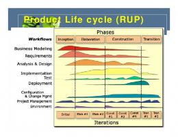
Product life cycle model.

in proposed bills of materials developed in the design phase can help designers determine designs that have lower risk of component obsolescence and therefore reduce the lifetime cost impact. In addition, obsolescence forecasting can be used throughout a product’s life cycle to analyze predicted component obsolescence dates and find the optimal time to administer a product redesign that will remove the maximum number of obsolete or high obsolescence risk parts. A. Life Cycle Forecasting The key benefit of life cycle forecasting is that it allows analysts to predict a range of dates when the part will become obsolete [2]. These dates enable project managers to set time frames for the completion of obsolescence mitigation projects; aid designers in determining when redesigns are needed; and enable managers to more effectively manage inventory. All of these effects of life cycle forecasting reduce the impacts of obsolescence [2]. Currently, most life cycle forecasting methods are developed based on the product life cycle model. As shown in Fig. 1, the model includes six stages: introduction, growth, maturity, saturation, decline, and phase out. When sales fall enough to be considered in phase out, many firms will discontinue the product, rendering it unsupported and obsolete. Solomon et al. [20] introduced the first obsolescence forecasting method that identified characteristics to estimate the life stage of a product. Characteristics such as sales, price, usage, part modification, number of competitors, and manufacturer profits, when combined, could estimate the stage and whether or not the product is close to phase out. However, the lack of a forecast indicating obsolescence in the immediate future is not useful for predictions of when, or if, a part might become obsolete in the long term [20]. One current method for life cycle forecasting utilizes data mining of sales data of parts or other elements and then fits a Gaussian trend curve to predict future sales over time [2], [19]. Using the predicted sales trend curve of a part, peak sales are estimated by the mean (denoted as μ in Fig. 2). Stages are then estimated based upon standard deviations (denoted as σ in Fig. 2) from the mean. Obsolescence forecasting predicts the zone of obsolescence. This zone is given between +2.5σ and +3.5σ and gives the lower and upper bound time intervals for when a part or element will become obsolete [19]. A potential shortcoming of this approach, however, is the assumption of normality of the sales cycle [19]. Another

This article has been accepted for inclusion in a future issue of this journal. Content is final as presented, with the exception of pagination. JENNINGS et al.: FORECASTING OBSOLESCENCE RISK AND PRODUCT LIFE CYCLE WITH MACHINE LEARNING

Fig. 2.

Life cycle forecast using Gaussian trend curve.

method involves organizing part information sales, price, usage, part modification, number of competitors, and manufacturer profits into an ontology to better estimate the current product life cycle stage of the part and then fit a trend line using current sales to predict future sales [21]–[23]. The zone of obsolescence is estimated using the predicted future sales, but does not assume normality since the factors utilized in the Gaussian trend curve [25] are used to estimate the stage, not the curve shape. Currently, most life cycle forecasting methods in the literature are built upon the concept of product life cycle model. This method involves data mining parts information databases for introduction dates and procurement lifetimes to create a function with the input being the introduction date and the output being the estimated life cycle [13]. The advantage of this method is the lack of reliance on sales data, the ability to create confidence limits on predictions, and the simplicity of a model with one input and one output [13]. However, this does not take into account the specifications of each individual part. As a result, the model could be skewed. For example, two manufacturers with two different design styles both make similar products. The first manufacturer creates a well-designed product and predicts that the specifications will hold in the market for five years. The second manufacturer does not conduct market research and introduces a new product every year to keep specifications up to market standards. Over the next five years, the first company will have one long life data point and the second company will have five short life data points; this will skew the model into predicting that the approximate life cycle is shorter than it actually is because the model does not take into account specifications. B. Obsolescence Risk Forecasting Another common method used for predicting obsolescence is obsolescence risk forecasting. Obsolescence risk forecasting involves creating a scale to indicate the levels of the chance of a part or element becoming obsolete. The most common of these scales is to use probability of obsolescence [15]–[18]. These scales, like product life cycle stage prediction, use a combination of key characteristics to identify where the part falls on a scale. Currently, two simple models exist for obsolescence risk forecasting; both use high, medium, and low ratings for key obsolescence factors that can identify the risk level of a part becoming obsolete [15], [16], [18]. Rojo et al. [18] conducted a survey of current obsolescence analysts and created an obsolescence risk forecasting best practice that looks at

3

numbers of manufacturers, years to end of life, stock available versus consumption rate, and operational impact criticality as key indicators for potential parts with high obsolescence risk. Josias and Terpenny [16] also created a risk index to measure obsolescence risk. The key metrics identified in this technique are manufacturers’ market share, number of manufacturers, life cycle stage, and company’s risk level [16]. The weights for each metric can be altered based on changes from industry to industry. However, this output metric is not a percentage, but rather a scale from zero to three (zero being no risk of obsolescence and three being high risk). Another approach introduced by van Jaarsveld uses demand data to estimate the risk of obsolescence. The method manually groups similar parts and watches the demand over time [17]. A formula is given to measure how a drop in demand increases the risk of obsolescence [17]. However, this method cannot predict very far into the future because it does not attempt to forecast out demand, which causes the obsolescence risk to be reactive. C. Obsolescence Forecasting Scalability For a method to be scalable, the framework must have the ability to adjust the capacity of predictions with minimal cost in minimal time over a large capacity range [22]. To achieve scalability in industry, obsolescence forecasting methods must meet the following requirements. 1) Do Not Require Frequent (Quarterly or More Often) Collection of Data for All Parts: The reason for this requirement is that many methods involve tracking sales data of products to estimate where the product is in the sales cycle [2], [19], [20]. A relatively small bill of material with 1000 parts would require a worker to find quarterly sales for 1000 parts and input them every quarter (or even more frequently). Companies have built Web scrapers to aggregate these data automatically, like specifications and product change notifications, but many manufacturers do not publish individual component sales publicly on the Web. Large commercial parts databases have contracts with manufacturers and distributors to gain access to sales data, but many companies not solely dedicated to aggregating component information have difficulty obtaining this information. The lack of ability of most companies to gather sales data makes forecasting methods requiring sales of individual parts extremely difficult to scale. 2) Remove All Human Bias About Markets: Asking humans to input opinion on every part leads to methods that are impractical for industry. In addition, finding and interviewing subject matter experts for long periods of time can be costly. Also, there may exist biases inherent in subject matter experts when estimating obsolescence risk within their field of expertise. These biases are largely due to experts being so ingrained in the traditions of their field that new products or skills can seem inferior when in fact they may supersede the expert’s traditional preferences. 3) Account for Multifeature Products in the Obsolescence Forecasting Methodology: Methods have been developed to predict obsolescence of single-feature products [2], [19], for example, flash drives. The flash drive may vary slightly in

This article has been accepted for inclusion in a future issue of this journal. Content is final as presented, with the exception of pagination. 4

IEEE TRANSACTIONS ON COMPONENTS, PACKAGING AND MANUFACTURING TECHNOLOGY

size and color but only has one key feature, memory. When a flash drive does not have sufficient memory to compete in the flash drive market, companies phase out that memory size in preference for ones with larger memory. Creating models for single-feature products like memory is straightforward because the part has only one variable that only causes one type of obsolescence, technical. However, multifeature products, for example, a car, can have many causes for becoming obsolete, and this makes it much more challenging to model. Some examples might include: 1) style obsolescence that comes from changes such as eliminating cigarette lighters, ashtrays, and the removal of wood paneling from the sides of cars; 2) the functional obsolescence of cassettes, and now even CD players for MP3 ports or Bluetooth; and 3) the technical obsolescence of drum brakes giving way to safer and longer running disk brakes. With these multiple obsolescence factors, many of the current forecasting models fall apart. Any obsolescence forecasting method that does not meet the three requirements described above will most likely develop problems when trying to scale to meet the needs of industry. Table I provides an overview of obsolescence forecasting methods that have been published in the last 15 years. Each method is characterized according to the type of obsolescence forecasting and whether it meets each of the scalability factors. Ideally, methods that do not require sales data or human input but should be capable of forecasting obsolescence for multifeature products. These characteristics are also indicated in Table I for each method. As shown, Sandborn et al.’s [13] is the only current method that does not require sales data or human inputs but does consider multifeature products. It creates a prediction model to predict lifespans of current products based on the past lifespans of similar parts, taking into account life cycle differences between manufacturers. However, this approach does not take into account the feature specifications of the part when predicting obsolescence dates. For example, one would expect that if two similar products are introduced into a market at the same time, and one is far more technically superior, the technically superior product would have a longer life cycle since it would be technically competitive in the market for a longer period. Without taking this technical progression into account, one of the key causes of technical obsolescence could be overlooked, leading to a potential decrease in accuracy of the model. D. Commercial Obsolescence Forecasting Services Because obsolescence forecasting can realize enormous cost savings for organizations, there are several companies that have emerged in recent years offering obsolescence forecasting and management as a service. Currently, some of the leading obsolescence forecasting and management companies include SiliconExpert, IHS, Total Parts Plus, AVCOM, and QTEC Solutions [23]–[27]. These companies focus on electronic components because of the high rate of obsolescence and have databases with information on millions of electronic parts such as part ID, specifications, and certification standards. The commercial forecasting services can be sorted into life cycle and obsolescence risk. Currently, SiliconExpert, Total Parts Plus, AVCOM, and QTEC Solutions offer life cycle forecasts,

Fig. 3.

Supervised learning process.

and IHS offers an obsolescence risk forecasting solution. However, none of these services offer both obsolescence risk and life cycle forecasting. III. M ETHODOLOGY In this section, two separate obsolescence forecasting methodologies and frameworks are introduced. Both approaches apply machine learning to improve accuracy and maintainability over other existing methods. The two approaches are differentiated by the two major outputs of the model. The first outputs the risk level that a product or component will become obsolete. This is termed ORML. The second method outputs an estimation of the date the product or component will become obsolete and is termed LCML. Machine learning has gained popularity in many application fields because it can process large data sets with many variables. The applications of machine learning range from creating better recommendation systems on Netflix to facial recognition in pictures to cancer prediction and prognosis [29]–[31]. Specifically, in the field of design, machine learning has been used to gather information and develop conclusions from previously underutilized sources. For example, public online customer reviews of products are mined to better understand how customers feel about individual product features [32]. The results of these analyses can be used to improve products during redesign and in new product development by understanding customers’ preferences in products. Another example of data mining and machine learning in design is the analysis of social media for feedback on products. Current work has shown that by using social media data, machine learning can predict sales of product and levels of market adoption [33]. Understanding the market adoption of features can indicate if the feature is a passing or a permanent trend. Both ORML and LCML use a subset of machine learning called supervised learning. Supervised learning creates predictive models based on data with known labels. These predictive models are used to predict labels of new and unknown data. A common introduction problem in supervised learning is to create a model to predict whether an individual will go outside or stay inside based on the weather. Two data sets are presented and follow the process shown in Fig. 3. The first data set contains the temperature, humidity, and sunniness for each day and whether the subject stayed inside or went outside. This data set is the training data set because a predictive model with output, stay inside or go outside, will be trained using these data. The training data set is fed into a

This article has been accepted for inclusion in a future issue of this journal. Content is final as presented, with the exception of pagination. JENNINGS et al.: FORECASTING OBSOLESCENCE RISK AND PRODUCT LIFE CYCLE WITH MACHINE LEARNING

5

TABLE I L IST OF A LL M ETHODOLOGIES AND S CALABILITY FACTORS

machine-learning algorithm, which creates a predictive model that will most accurately classify the known label based on the known weather information. The new model can also be fed weather information where the label is unknown. The model will predict the label with the highest likelihood of occurring. The unknown data set is also called the test set because it will be used to test the accuracy of the predictive model. For the stay-inside-or-go-outside prediction model and all supervised learning models, the more the data with known labels submitted to the machine-learning algorithm, the more effective the predictive model. This means supervised machine learning is a strong fit for any problem where data continually flow in and can make the predictions more accurate. With prediction of product obsolescence, the stream of newly created and discontinued products allows the predictive models created using ORML and LCML to gain accuracy over time. Supervised machine learning was chosen over unsupervised machine learning because the latter does not have a known data set. Unsupervised machine learning does not have a label to predict, but rather uses algorithms to fix clusters and patterns in the data. Similar methods could be advantageous to identifying groups of comparable products for product redesign or for cost reduction in the design phase. However, due to unsupervised machine learning finding groupings that are not explicitly obsolete versus active, supervised learning was chosen over unsupervised learning for this obsolescence forecasting framework. In addition, machine learning models are not deterministic models. Many algorithms use randomization to split variables and evaluate the outcome. A byproduct of this trait is that the predictive models will vary slightly each time the algorithm is implemented. Even with these slight variations, machine learning models are highly effective and used in many predictive applications. A. Obsolescence Risk Forecasting Using Machine Learning The forecasting methods introduced and demonstrated in this paper are based on the concept that parts become

Fig. 4.

Outputs of ORML.

obsolete because other products in the market have a superior combination of features, software, and/or other added value. The ORML framework, like the weather example, is shown information and attempts to classify the part with the correct label. However, instead of weather information, the technical specifications of current active and obsolete parts are fed into algorithms to create the predictive models. In Fig. 3, after the predictive model is created, the technical specifications of parts with unknown obsolescence statuses are structured in the same way as that for the known parts and input to the predictive model. The model outputs the probability that the part is classified with the label active or obsolete. The probability that the part is obsolete can be used to show the obsolescence risk level. Fig. 4 shows the output from the ORML method. Product A shows a product with a 100% chance of the part being active. Product B demonstrates a mixed prediction with between a 60% chance of being active and a 40% chance of being obsolete. Product C shows the prediction of a product with a 100% chance of being obsolete. One application of this output is to predict the obsolescence risk level for every component in two competing designs or subassemblies and then create a composite obsolescence risk level for each design using a combination of the components’ risks. The new composite risk level could be used as an attribute in the process for selecting a final design.

This article has been accepted for inclusion in a future issue of this journal. Content is final as presented, with the exception of pagination. 6

IEEE TRANSACTIONS ON COMPONENTS, PACKAGING AND MANUFACTURING TECHNOLOGY

B. Life Cycle Forecasting Using Machine Learning The LCML framework is built on the same principle that parts become obsolete because other products in the market have a superior combination of features, software, and/or other added value, the difference being what the frameworks are predicting. Where ORML predicts the label active or obsolete, LCML uses regression to predict a numeric value of when the product/component will stop being manufactured. LCML’s ability to estimate a date of obsolescence is a highly useful metric. LCML will give designers and supply chain professionals a more effective way of predicting the length of time to complete redesign or find a substitute supplier or component. Understanding when each component on a bill of materials will become obsolete will allow designers the ability not only to provide time constraints on projects, but also more effectively time redesign projects to maximize the number of high risk components removed from the assembly. The combinations of the ORML and LCML outputs in analyses have numerous applications in business decision making processes. Current commercial obsolescence forecasting methods and those in the literature only predict obsolescence risk or product life cycle. Since the ORML and LCML models both use product specifications as input and the same machinelearning algorithms to build the model, the only additional work needed to switch between predicting risk versus life cycle is changing the output in the training data. This is just one of the reasons a machine learning-based obsolescence forecasting method is superior. Currently, it is the only method that readily provides obsolescence risk and product life cycle, essential to improve accuracy. IV. C ASE S TUDY The case study serves to demonstrate the accuracy and scalability of ORML and LCML as methods to forecast obsolescence. The cell phone market was chosen for the case study due to availability of data and the ease it provides in understanding the product and specifications. Although the case study is a consumer product, the ORML and LCML prediction frameworks can be utilized to predict component obsolescence found in larger complex systems. The case data contain over 7000 unique models of cellular phones with known procurable or discontinued status, release year and quarter, and other technical specifications. The specifications include weight (g), screen size (in), screen resolution (pixels), talk time on one battery (min), primary and secondary camera size (MP), type of Web browser, and if the phone has the following: 3.5-mm headphone jack, Bluetooth, e-mail, push e-mail, radio, SMS, MMS, thread text messaging, GPS, vibration alerts, or a physical keyboard. The data set included 4030 procurable and 3021 discontinued phones. However, the data set only included 38 obsolescence dates. This means that the ORML portion of the case study had 7051 unique cell phone models while the LCML had 38. Although the data sets differ in size, each data set is suitable in size to demonstrate the ORML and LCML frameworks. The data were collected from one of the most popular cell phone forums, GSM Arena, using a Web scraper. The original

TABLE II N EURAL N ETWORKS ORML C ONFUSION M ATRIX FOR C ELL P HONES

TABLE III SVM ORML C ONFUSION M ATRIX FOR C ELL P HONES

data set, and the code for the Web scraper, and machine learning models created in this case study can be downloaded from connorj.github.io/research. GSM Arena is an online forum that provides detailed and accurate information about mobile phones and associated features. For this reason, the data set can have missing values and even miss reported information. Even with these shortfalls with the data set, this more accurately represents data collected in industry and demonstrates the robustness of the ORML and LCML frameworks. After formatting the data, the data set was split into two random groups. The first group represents 2/3 of the data set and is called the training data set. The training set is the data set used to create the prediction model. The second is the test set and represents the other 1/3. Although all the data sets are known in this case study, the test set will be put through the predictive model, and accuracy will be determined by comparing actuals obsolescence statuses and obsolescence date with the one predicted by the model. This practice is known as validation and is a best practice for model creation and evaluation because the data used to create a prediction model are never used to validate its accuracy [34]. Currently, the majority of the obsolescence forecasting models in the literature estimate model accuracy by using the same data used to create the model. The data set was split into a 1/3 test set and a 2/3 training set for an initial analysis for accuracy using confusion matrices. A more indepth analysis was conducted where the ratio of training and test set sizes was changed and the accuracy was assessed (Tables V and VII) [35]. The next step in the case study was to run the training data set through a machine-learning algorithm to create a predictive model. Machine learning has many algorithms and infinitely more if counting all the slight variations that can be done to increase accuracy. Three machine-learning algorithms, artificial neural networks (ANNs), support vector machines (SVMs), and random forest (RF) will be applied to this case study [36]–[38]. Decision trees and SVMs were ranked first and third, respectively, on the list of top

This article has been accepted for inclusion in a future issue of this journal. Content is final as presented, with the exception of pagination. JENNINGS et al.: FORECASTING OBSOLESCENCE RISK AND PRODUCT LIFE CYCLE WITH MACHINE LEARNING

7

TABLE IV RF ORML C ONFUSION M ATRIX FOR C ELL P HONES

Fig. 5. Overall average evaluation speed by the training data set fraction for ORML.

ten algorithms in data mining [39]. However, standard decision trees are often inaccurate and overfit data sets [41]. RF, an aggregation of many decision trees, averages the trees with the intention of lowering the variance of the prediction [41]. For this reason, RF was selected over standard decision trees. The algorithm listed second, K-means, is an unsupervised clustering method and would group similar products together rather than forecast an output. For this reason, K-means is not a possible alternative for an algorithm to be used for either ORML or LCML and therefore was not included in this case study. Although ANNs were not on this top 10 list, they were selected based on wide usage in deep learning, a subset of machine learning. Deep learning looks at the complex relationships between inputs in an effort to have a greater understanding of combined relationships with the output [41]. In the final step, once the algorithm constructs a predictive model, each part or element from the unknown data set is run through the model and receives a predicted label. A. Results of Obsolescence Risk Forecasting The accuracy of the ORML model is represented in a confusion matrix. The confusion matrix (Tables II–IV) shows how many cell phones were classified correctly versus those classified incorrectly. Numbers in the (available, available) and (discontinued, discontinued) cells are correctly classified and all other cells are misclassified. The first algorithm used was ANN. The neural networks classification was done in R 3.0.2 using the package caret [40]. All the ANNs in this study were constructed with two hidden layers. The probability of each part being available or discontinued was output, and the highest probability label of available or discontinued was assigned. The actual statuses were compared to the predicted values, and a confusion matrix was developed (Table II). The model correctly predicted 91.66% of cell phones with the correct label in the test data set. The next algorithm applied was SVM. The SVM utilized the SVM classification function from the package e1071 [41] in R 3.0.2 and a radial basis kernel was selected. The algorithm was implemented on the training data set that contained 66.6% of the total data. The prediction model then classified the remaining 33.3% of phones not used in the model creation. The actual statuses and the predicted statuses were compared, and the confusion matrix in Table III was created. The SVM model has a model accuracy of 92.4%. The last algorithm applied was RF. The model was implemented in R 3.0.2 using the package randomForest [42]. The randomForest function was set to have 500 trees for all RFs in this case study. The model was trained with a 66.6% training

set and was tested with 33.3%. The predicted test set and the actual statuses are compared in Table IV. The model received an accuracy of 92.56%. This was the highest of all three algorithms. For Tables II–IV, the training size was held constant at 66.6%. Table V illustrates how changing the percent of instances from the data set used to create the model affects accuracy. ANN and SVM preform at about the same accuracy for every training size, while RF always performs at a higher accuracy. The algorithms were compared using the prediction model creation time for each of the 50%–100% training sets used in Table V. Ten predictive models were created for each training size, and the average time was plotted (Fig. 5). All the algorithms increased in time at a near constant rate. ANN is the fastest algorithm, followed by SVM, which is followed by RF. Although the speed of creating these predictive models is relatively small (