Forecasting Requirements in the Optimal Control

Forecasting Requirements in the Optimal Control of Wave Energy Converters Francesco Fusco January 2009

Research Report: EE/2009/2/JVR Department of Electronic Engineering, NUI Maynooth Maynooth, Co. Kildare, Ireland

Contents 1 Introduction

2

2 Conditions for optimality

3

3 Practical realisation of optimal conditions through 3.1 Time series forecasting and predictability . . . . . . 3.2 Forecasts based on deterministic physical laws . . . . 3.3 Forecasting error effects and error rejection . . . . .

control . . . . . . . . . . . . . . . . . . . . .

5 10 13 15

4 Main forecasting approaches related to wave energy optimisation 4.1 Wave pressure estimation by the Kalman Filter . . . . . . . . . . 4.2 Deterministic sea wave prediction . . . . . . . . . . . . . . . . . . 4.3 Digital filters for wave forecasting . . . . . . . . . . . . . . . . . . 4.4 Spatial wave forecasting through a linear harmonic model . . . . 4.5 Non-linear next wave estimation . . . . . . . . . . . . . . . . . .

18 18 20 21 23 24

5 Conclusion

26

6 Acronyms

29

1

1

Introduction

A large number of proposed devices for wave energy extraction consists of oscillating systems, which could be in the form of bodies oscillating with respect to a fixed reference, multiple bodies oscillating relatively to each other, or also oscillating water columns (OWC) [1]. In the first two cases the mechanical energy stored, in the form of mixed potential and kinetic energy, in the whole oscillating system is then converted to useful energy by means of some power take off device. In OWC systems, on the other hand, the incident waves produce the oscillation of the water column in a chamber, where a dynamic pressure is consequently generated, if the chamber’s volume is not too large. The energy stored in this dynamic (oscillating) air pressure in the OWC chamber is then turned into useful energy most commonly by means of pneumatic machinery (but also hydraulic takeoff devices may be used)[2]. Theory exists about optimising the energy extracted from the waves by means of such oscillating systems, and it emerges from it that future knowledge of certain physical quantities is required for the optimisation conditions to be achieved. These quantities may be the wave excitation force or the oscillation velocity in the case of oscillating bodies, excitation volume flux or air chamber pressure in the case of oscillating water columns. To approach as much as possible the optimality conditions, in practise, it is therefore necessary that a prediction for some time into the future of some of those physical quantities is provided. All of these quantities are, however, strictly dependant (sometimes even through a non-causal transformation) on the incident wave so that the problem of wave forecasting becomes central in this context [1],[3]. It is worth mentioning also that solutions of the overtopping type, for the extraction of energy from ocean waves, were also proposed. Here, by means of hydro turbines, the energy is extracted from the potential energy stored in the water coming from the overtopping of waves up to a ramp and then into a reservoir [4],[5]. The nature of this solution, however, does not allow (or at least did not allow so far) a full comprehensive general theory from where conditions of optimality or ideal solutions to the problem could be drawn, like in the aforementioned case of the oscillating systems. Even in this case, however, short term wave forecasting, which would allow the prediction of the overtopping water flows, appears to be a most relevant possibility to achieve energy capture improvements [6],[4]. This report is proposed as an analysis about this necessity of prediction and its impact on the design procedure of a general control framework when a prediction error is considered. Section 2 provides an insight over the general optimal conditions for the wave energy extraction by means of oscillating systems, based on linear theory. Then, the practical issues involved in the design of a real control architecture trying to realise these conditions are discussed in section 3. Section 4 outlines the main approaches present in the scientific literature, concerning wave prediction related to wave energy extraction improvement. Finally, areas of study involving further directions of investigation are documented in the conclusion, section 5.

2

2

Conditions for optimality

Optimal conditions for the maximisation of wave energy extraction, by means of oscillating systems, are described in detail by Falnes [2], where linearity is assumed. For the case of a single oscillating body in one single degree of freedom (which may either be heave, pitch or whatever else), the following alternative optimality conditions apply: u(ω) =

Fe (ω) 2Ri (ω)

(1)

, which here will be termed the phase and amplitude condition, and Fl (ω) = −Zi∗ (ω)u(ω)

(2)

termed the reactive condition or the complex-conjugate condition. Condition (1) furnishes the optimal oscillation velocity u(ω) for the body to achieve maximum energy absorption from the incident wave, producing an excitation force Fe (ω) on the body itself (it is the force that the wave would produce if the body was not moving, as its motion produces a radiation force as well, due to the radiated waves). The quantity Ri (ω) is the real part of the intrinsic mechanical impedance of the body, defined as Zi (ω) , [Fe (ω) + Fl (ω)] /u(ω), with Fl (ω) a generic load force provided by a power take-off device. Before further commenting on this and the following conditions, however, it is important to clarify that they are not exact as they were derived under some simplifying assumptions of linearity, as mentioned before, which should be kept in mind. First of all, linearity is assumed in the sense that a harmonic signal in the original source (the wave) produces a perfectly harmonic effect on the body (wave excitation force, velocity) with the same frequency as in the input. That is, denoting by u(t) and y(t) a generic input and response respectively, and indicating as =(·) the input-output mapping, the following is supposed: u(t) = ρu sin(ωt + ϕu ) =⇒ y(t) = = [u(t)] = ρy sin(ωt + ϕy )

(3)

where ρu and ρy represent real quantities, so that only a change in the amplitude and phase may occour between the input and the output. Another important simplifying assumption which has to be pointed out is the extension to the frequency domain ω, only possible if several harmonic components acting together are supposed to be completely independent in the source (still the wave) and at the same time are supposed to map completely independently to each other in the same frequency of the effects (excitation force, velocity). That is, the superposition principle is assumed to be valid: X X   ρu,i sin(ωi t + ϕu,i ) ρy,i sin(ωi t + ϕy,i )  u(t) =  y(t) = = [u(t)] = =⇒ i i   ui (t) = ρu,i sin(ωi t + ϕu,i ) yi (t) = = [ui (t)] = ρy,i sin(ωi t + ϕy,i ) (4) In reality, of course, such a behaviour rarely exists, but these simplifications allow an analytical treatment of the problem which, although not exact, is still valuable in providing conditions and considerations which will be fundamental in practise, as we will see in the following. 3

Going back to the phase and amplitude condition (1), it puts a constraint on the optimal velocity to be in phase with the wave excitation force (Ri is a real quantity) and to assume a certain amplitude (from where the name attached to this condition derives). A control system trying to achieve this condition, where the reference will therefore be this optimal velocity, is termed an optimal phase and amplitude control. It can be shown that the amplitude condition is an active condition, in the sense that it requires that energy is provided to the system in part of each cycle, so that it implies significant difficulty to be implemented efficiently. That’s why some control systems were developed, where only the achievement of the passive (but sub-optimal) phase condition is attempted, the most famous of them being latching control (e.g. refer to [7],[8],[9]). The complex-conjugate condition (2), on the other hand, expresses an optimal relationship between the load force Fl (ω), provided by a certain power take-off machinery, and the oscillation velocity of the body u(ω). The two quantities are related by the load impedance Zl (ω) , −Fl (ω)/u(ω) and, in order to achieve optimality, as a consequence of condition (2): Zl (ω) = Zi∗ (ω)

(5)

that is the load impedance should equal the complex conjugate of the intrinsic mechanical impedance Zi (ω) of the system. A control system which acts on the load impedance, on the basis of a reference being the optimal load force Fl (ω), in order to obtain the maximum energy absorption, is termed reactive control or complex-conjugate control for obvious reasons and it is interesting to note how it is perfectly analogue to the problem of impedance matching, typical of electrical circuits. In the most general case of multi-body oscillating systems with more than one degree of freedom, an optimal condition was also derived and it is summarised in [2] as: 1 (6) u = R−1 Fe 2 where underlined bold symbols represent vectors and bold symbols denote matrices. Here the components of u are the oscillation velocities of each body in each direction of motion, R is the real and symmetric radiation-resistance matrix of the system and Fe contains the excitation forces acting on each body and along each degree of freedom. It is not in the interest of this author to detail all the implications that were derived from such a condition, but the important thing that will be pointed out is that there is no longer a phase condition between the oscillation velocity of each body along some particular direction and the excitation force acting on that same body along the same direction. The non-diagonal elements of R, in fact, force the optimal velocities to be a linear combination of the wave excitation forces acting on all the bodies and in all the directions (in the most general case). In the remainder of this report, only the one degree of freedom case will be considered for the sake of simplicity, as it is sufficient for our purposes, but it is worth pointing out that energy extraction optimisation in the most general case (when oscillating bodies are considered) requires a specific relationship between oscillating velocities and wave excitation forces to be satisfied. As mentioned in the introduction, wave energy extraction by oscillating systems may also be realised through oscillating water columns (OWCs) instead 4

of oscillating bodies. In this situation, two alternative optimal conditions, analogue to (1) and (2), were derived [2]: Qe (ω) 2G(ω) Ql (ω) = Y ∗ (ω)p(ω) p(ω) =

(7) (8)

The first condition (7) relates amplitudes and phases of the dynamic air pressure inside the chamber p(ω) and the excitation volume flow due to the incident wave Qe (ω). The quantity G is the radiation conductance of the OWC system, that is the real part of the radiation admittance, defined as Y (ω) , −Qr (ω)/p(ω), with Qr (ω) being the radiated volume flow from the OWC chamber. As regards equation (8), it is analogue, in some ways, to the complexconjugate condition (2) as it states that, in order to achieve optimality, the load admittance Λ(ω) , Ql (ω)/p(ω) of a generic power takeoff device shall equal the complex conjugate of the OWC chamber radiation admittance Y (ω). Conditions for systems constituted by several OWCs or by combinations of oscillating bodies and OWCs may be derived, but the substance of them, in our purposes, is always that some relationships between the introduced physical quantities need to be satisfied.

3

Practical realisation of optimal conditions through control

Given the conditions according to which the system will be in an optimal state, in the sense of absorbed energy from the incoming waves, the practical way to make sure that it will always tend to that state during its operational functioning period, is by means of control. A property of the system is therefore controlled in order to be as close as possible to some reference signal calculated on the basis of some of an optimal condition, by means of a controller (normally a digital algorithm) acting on the system through a certain input signal. This most general approach may be schematised, for the sake of clarity, as in figure 1. A reference model provides, at each instant (or at each sampling instant in the case of a digital implementation), the optimal reference ropt (t) for the controlled variable y(t) on the basis of some measurements iref (t). Then, a controller decides the appropriate input for the system i(t) based on the error e(t) between the optimal reference and the current controlled variable value. Depending, of course, on the nature of the system, on the available measurements and on the choice for the inputs/outputs of the system, this general control architecture will identify itself with a more specific structure where each of the individuated signals will assume a precise physical significance. The four optimality conditions (1), (2), (7) and (8), outlined in section 2, provide at least four corresponding possibilities in choosing the physical quantity to control, and each possibility may give raise to several control architectures. In particular, these quantities may be the oscillating body’s velocity or the load force provided by the power take-off device in the case of an oscillating body, whose reference would be given by conditions (1) and (2), and dynamic air

5

iref

reference model

ropt + −

e

controller

i

system

y

y

Figure 1: A wave energy absorber (system block) may achieve its optimal energy extraction condition, in practise, if a proper control system is designed. η

Hf e(ω)

Fe

1 2Ri (ω)

uopt + −

controller

Fl

system

u

u

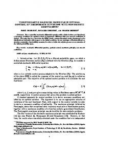
Figure 2: Oscillation velocity of the body is the controlled variable. Wave excitation force calculated by means of wave elevation observations. pressure in the chamber or the water volume flow at the load for the case of an OWC, which would be regulated on the basis of conditions (7) and (8). As an example, consider the three possible control schemes in figures 2, 3 and 4, the first two representing two alternatives for the application of condition (1) and the third one being a possible approach to the realisation of condition (2), as firstly proposed in [2]. For the control system in figure 2, the controlled variable is the oscillation velocity of the wave energy converter and a generic controller, acting on the system through a load force Fl , is designed in order to make it assume the optimal value, denoted uopt , calculated from optimal condition (1). In order to compute this reference signal, knowledge of the wave excitation force Fe acting on the system is required, which here is assumed to be calculated from incident wave measurements. Figure 3 presents the same approach but with the excitation force estimated from measurements of the total wave force acting on the system and then corrected on the basis of the radiation force (here assumed to be calculated as Fr = Zr u, with Zr representing a radiation impedance). Finally, in the control scheme 4, the the load force given as input to the system is directly calculated from condition (2) by means of oscillation velocity measurements. Note that in the three schemes the load force is supposed to be an input to the system, but this does not mean that we can act directly on it, so that in general a further (more then one) control loop is expected to be present into the block

Fw

Fe

+ −

Fr −Zr (ω)

1 2Ri (ω)

uopt + −

controller

Fl

system

u

u

u

Figure 3: Oscillation velocity of the body is the controlled variable. Wave excitation force calculated by means of total wave force measurements. 6

u

Fl,opt

−Zi∗ (ω)

u

system

Figure 4: Load force is the controlled variable, and its optimal value is directly derived from oscilaltion velocity measurements through the reactive condition (2). termed system. Note, moreover, that these are only some sample possibilities and different alternatives (although always equal in the optimality principle) could be figured out, but this is more than enough, in the author’s opinion, to provide motivations for the necessity (as mentioned in the introduction) of predicting some key physical quantities for practical implementations. The blocks in these control schemes have been expressed as transfer functions in the frequency domain, as also were the optimal conditions outlined in section 2 but, in reality, computations need to be made in the time domain. In the time domain it turns out that some of the blocks are constituted by noncausal transfer functions, unfeasible in practise as future knowledge of their input variable is required to compute their output. In particular, non causality affects the kernel functions of the following relationships: Z +∞ Fe (ω) ⇐⇒ uopt (t) = hu (t − τ )fe (τ )dτ (9) uopt (ω) = 2Ri (ω) −∞ Z +∞ Fe (ω) = Hf e (ω)η(ω) ⇐⇒ fe (t) = hf e (t − τ )η(τ )dτ (10) −∞

Fl,otp (ω) = −Zi∗ (ω)u(ω) ⇐⇒ fl (t) =

Z

+∞

hf l (t − τ )u(τ )dτ

(11)

−∞

where 

1 2Ri (ω)



,

non causal

(12)

hf e (t) = F −1 {Hf e (ω)} ,

non causal

(13)

{−Zi∗ (ω)} ,

non causal

(14)

hu (t) = F −1

hf l (t) = F

−1

Proof for non causality of these impulse reponse functions is provided by Falnes [2],[3]. As regards hu (t), in fact, it corresponds to the inverse Fourier transform of the real even function 1/2Ri (ω) (again, refer to [2],[3] for justifications about the intrinsic mechanical resistance being an even function) and, for the properties of the Fourier transform, it is even itself and therefore non-causal (non-zero for negative values of t). With regard to hf l (t), it may be written, on the basis of some Fourier transform properties: hf l (t) = F −1 {−Zi∗ (ω)} (t) = −F −1 {Zi (ω)} (−t)= ˆ − zi (−t)

(15)

The inverse Fourier transform of the intrinsic mechanical resistence Zi (ω), however, here named zi (t), is definitely causal (refer to [2]) and therefore hf l (t) is 7

non-causal (being zero for any t > 0). Non-causality of the impulse response function hf e (t), relating the wave excitation force to the incident wave may also be demonstrated, and it can be interpreted by thinking of the wave exerting some influence on the system before actually coming in touch with it. Analogue procedures lead to the demonstration of the practical infeasibility of the computation, at any time instant, of optimal conditions (7) and (8) found for the case of an oscillating water column. Optimality, however, although impracticable, may be approached by forecasting the physical quantity of interest. Forecasts, however, will never be exact and surely the prediction error will be larger the further into the future the forecasting horizon extends. Regardless of the specific algorithm utilised to extrapolate the future behavior of a certain physical quantity, there will inevitably be, in fact, an upper bound to the overall achieveble performance, which will strictly be dependant on the availability and the accuracy of the measurements of the quantities somewhat related to it, and on its coherence time, auto-correlation or cross-correlation with the measured signals. That’s why the different control strategies, which all theoretically realise the same optimum condition of maximum energy extraction, may perform totally differently in the reality due to the aforementioned practical infeasibility. Jumping back to the three sample control architectures of figures 2 to 4, let’s try to figure out what the introduction of predictions, in order to make them realisable, implies. Note that all of the non-causalities appear in what may be referred to as the reference model, that is where the reference signal for the actual control system is generated. In the first case, the wave excitation force is supposed to be calculated from wave measurements. But in order to determine the optimal reference oscillation velocity for the absorber, future values of the excitation force are required, so that either the wave excitation force is predicted on the basis of its current and past values or calculated on the basis of future wave elevation predictions. As it was mentioned before, however, even the current wave excitation force depends on future wave elevations, so that wave forecasting is required in any case, unless one decides to forecast both current and future excitation force values on the basis of the most recent values that it is possible to calculate from the available wave observations. We have supposed, however, that the wave observations were taken at the exact point of the sea surface where the wave energy converter is placed. But this assumption may not be achieved in practise so that the wave should be measured at some distance from the device (such a choice may also be undertaken only due to reasons of effectiveness of the solution). This fact implies several things. If it is decided to follow the approach of forecasting the wave, a more deterministic approach may be utilised in order to calculate the future incident wave, from knowledge on its spatial propagation laws. This may provide more accurate predictions and for longer time horizons than simply extrapolating future wave elevations based on past observations collected at the same point, which would be a purely stochastic approach and which would provide a lower bound on the achieavble prediction error depending on the coherence time of the wave or on its autocorrelation, as mentioned before. Spatial prediction (point to point prediction) of the wave, however, may present some problems: 1. The transfer function relating the wave elevation at two points of the sea

8

surface on the propagation direction of the wave, where the downstream point is considered as output, is non-causal unless a sufficiently long distance is considered, and this is due to the dispersive characteristic of sea waves propagation (as will be discussed in 3.2); 2. The wave excitation force depends exclusively on the incident wave of the body and not on the radiated wave (a still body is supposed in the definition of excitation force), so that unless the observations are taken sufficiently far away from the device so that the radiated wave may be neglected, an algorithm to separate the incident wave from the radiated wave should be considered (like the one discussed in [10]); 3. Multi-directional waves may significantly increase the complexity of the problem, above all if the distance of the obseravtion point from the prediction site is large. The same problems appear when deciding to directly forecast the excitation force. In this case, in order to compute the most recent excitation force values as possible (depending on the non-causality of the transfer function) from wave measurements collected far from the wave absorber, we may still require the separation of incident wave from radiated wave and may also still be dealing with the problem of multi-directionality. Note also that, in this case, a more deterministic estimation of the future wave excitation force values may be obtained if wave elevation observations are collected further from the device (the transfer function becomes less non-causal with the distance). In the other approach, of figure 3, forecasting of just the wave excitation force is required, and it should be based on past observations of the excitation force itself, which are assumed to be computable from measurement of the wave force corrected on the radiation force (calculated through oscillation velocity measurements). This would be a purely stochastic approach and its performance still depends on the coherence time of the considered physical quantity (which may be longer than the coherence time related to the wave elevation signal at one point of the sea as there is some filtering effect between them, but this is only a qualitative statement based on intuition and it is not proven). Finally, the third control option presented, requiring the prediction of the WEC’s oscillation velocity. This implies several difficulties due to the fact that future oscillation velocity depends on future control decisions and not only on external factors (such as the incident wave). That is, the quantity to predict is not an independent variable, but it is a dependent variable and more precisely it is the controlled variable. It is interesting, at this point, discuss more into the details, the main points that emerged from these qualitative dissertation about the practical implications that the application of control theory to the optimisation of a wave energy converter involves. In particular, sections 3.1 and 3.2 will be aimed to give some more theoretical insight, respectively, on the two someway opposite problems of purely stochastic forecasts of a quantity exclusively based on its previous observations and deterministic forecasting exploiting physical laws relating different measurement points of the specific quantity. Then, section 3.3 will outline some of the possibilities of treating the inevitable forecasting error that will be present in the overall control flow, its effects on the control performance and how it can be limited by some sort of robust control. 9

3.1

Time series forecasting and predictability

One of the possibilities to design an optimal control framework for maximising the wave energy extraction of a wave energy converter, as emerged from the discussion of above, is through the prediction of a certain physical quantity simply based on information about its current and past behavior. The quantity may then be considered as a pure time series and the problem becomes its multistep ahead prediction, which is normally treated as a stochastic problem, even if some deterministic knowledge about the signal’s evolution may be included in the forecasting model. By considering this approach, we implicitly make the assumption that no other information about exogenous variables having some influence on the considered variable is known and, therefore, it must be possible to analyse what are the limitations in the forecasts accuracy independently on the actual technique which will be eventually utilised to compute them. This consideration derives from the fact that, obviously, any attempt to extrapolate the future behavior of the signal may not go beyond the maximum information that can be extracted from the present and from the past of the signal itself. It would be fundamental, therefore, trying to analyse and, in some ways, quantify, what may be considered as the predictability of the signal, that is its property of being predicted only from past values, which should be independent on a specific tool which is then utilised to actually achieve it. Such an important intrinsic property of a signal, or of a system more in general, has been studied in statistics and in information theory and it was quantitatively related to the entropy and to the mutual information respectively of a random process and between two random processes [11]. It is therefore worth providing a brief insight about the theoretical definitions of these quantities and their properties. Jones [12] gives the following definition for the self information, denoted by I(ei ), of a possible event ei of a system S constituted ba a set of n events {e1 , ..., en }, whose probabilities P {ei } = pi sum up to 1 (one event must always occour): I(ei ) , − log pi (16) where the logarithmic base is not specificed with the justification that it may be chosen appropriately according to the specific nature of the problem. In any case, however, the sense of this definition is that the rarer an event is (i.e. the smaller pi ) the more information is conveyed by its occourrence (i.e. the larger I(ei )). The self information is, in fact, bounded as follows: 0 ≤ P {ei } ≤ 1

=⇒

0 ≤ I(ei ) < +∞

(17)

The introduction of the self information property is fundamental in defining the entropy, which, as we will see, offers the possibility of quantifying the intrinsic uncertainty of a system and it becomes therefore central in our attempt to provide a measure for the predictability of a time series. Based on the property of the expectation operator E {·}, applied to a generic function f (·) defined in the system S, according to which: E {f } =

n X k=1

10

pk f (ek )

(18)

the entropy of the system S, denoted by H(S), may be defined as [12]: H(S) , E {I} = −

n X

pk log pk

(19)

k=1

The uncertainty arising when pk = 0 is bypassed by assigning the value 0 to pk log pk in such a circumstance. The reasons why entropy is a suitable measure for the uncertainty of the system are deduced from its following properties, which here are provided without proof (refer to [12] for details): 0 ≤ H(S) ≤ log n

(20)

H(s) = 0

(21)

⇐⇒

H(s) = log n

∃ ! k ∈ [1, n] : pk = 1 and pi = 0 ∀ i ∈ [1, n], i 6= k 1 ∀ k ∈ [1, n] ⇐⇒ pk = n

(22)

These properties define an upper and lower bound for the entropy and assert that it is minimum (null), according to (21), when only one event is possible so that there is certainty about the system, and it is maximum (log n), according to (22), when all the events are equally possible. Now that we have a way to quantify the overall unxcertainty intrinsic in a certain system (which may be a random process or a random variable in the statistics sense), we still need to understand if it is possible to determine and quantify how this uncertainty may be reduced on the basis of some information that we acquired about the system itself or about any related system. Information theory still turns out to be useful in this perspective, particularly with the concepts of conditional entropy and mutual information. In order to introduce these definitions, it is necessary to define two systems S1 = {e1 , ..., en } and S2 = {f1 , ..., fn } as sets of respectively n and m possible events whose probabilities, denoted respectively as pk , P {ek } and qk , P {fk }, sum up to one as well. The entropy of S1 , conditioned on S2 , and denoted by H(S1 /S2 ), is then defined as:   m n X X pjk pjk log H(S1 /S2 ) , − (23) qk j=1 k=1

where pjk , P {ej fk } is the joint probability between the events ej and fk the uncertainty appearing when pjk = 0 and qk = 0 (which implies pjk = 0) are resolved by putting pjk log(pjk /qk ) = 0, as for the entropy of a system. From its definition it is clear that the conditional entropy represents the uncertainty in system S1 when information about the system S2 is available, and in fact it may be shown that H(S1 /S2 ) is bounded as follows: T

0 ≤ H(S1 /S2 ) ≤ H(S1 )

(24)

where it is at its minimum when the events in S1 are perfectly associated to the events in S2 (no uncertainty) while it is at its maximum when the events in the two systems are completely independent (uncertainty about S1 does not decrease when knowledge about S2 is available). An alternative way to represent this concept is the mutual information I(S1 , S2 ) , defined as: I(S1 , S2 ) , H(S1 ) − H(S1 /S2 ) 11

(25)

which, in an opposite way to the conditional entropy, is maximum (H(S1 )) when the system S2 contains all the possible information about S1 and it is minimum (null) when information about S2 is totally uncorrelated to what happens in S1 . These very general concepts from information theory represent an interesting answer to the original question on whether it is possible to quantify how much information about the future behavior of a time series is contained in its past and current behavior so that it would be possible to determine how long in the future predictions will be effective and in what measure. Systems S1 and S2 may in fact represent, respectively, the future and the past behavior of the time series for any chosen number of samples. Note that these general measures may also be applied to the forecasting possibilities analysed in the next section 3.2, where predictions are based on observations of a different physical quantity or of the same one but at a different location. It may represent, therefore, a very useful tool in assessing the performance which is theoretically possible to achieve, independent of the particular forecasting algorithm utilised, for any different choice of the measured variables and the forecasted quantity. The problem lies in the actual possibilitiy of computing the mutual information index or the conditional entropy, which may be a very complex problem, as it requires computation of probability and conditional probability distributions of the involved variables. Particularly in the case of the time series forecasting, an alternative and more computationally effective predictability index, was derived in [13]. Denoted by R(k)2 , this index was defined as the ratio of the optimal prediction variance to the time series x(t) (assumed to have zero mean, without affecting the generality of the definition) variance, i.e.  E x ˆ(t + k/t)2 2 (26) R(k) , E {x(t)2 } where E{·} is the expectation value operator and x ˆ(t + k/k) is the optimal prediction (in the sense of minimising the prediction error variance) attainable from the observations of the time series until the instant k. From the properties of the optimal prediction, which is known to be orthogonal (uncorrelated) to the prediction error eˆ(k) = y(t + k) − yˆ(t + k/t), the predictability index R(k)2 may be alternatively expressed as: R(k)2 = 1 −

σk2 E{x(t)2 }

(27)

where σk2 = E{ˆ e(k)2 } is the variance of the prediction error. From this formulation it is straightforward to observe how the index is 1 (maximum) if the time series is perfectly predictable (null prediction error), whereas it is null (minimum) when the time series is completely unpredictable (prediction error equal to the time series). A quite effective (from a computational point of view) algorithm for the computation of this index is also provided in [13] and may represent a simpler and more direct alternative to the general measures from information theory, to asses the predictability of a time series (also depending on the forecasting time horizon) independently from any particular forecasting algorithm.

12

3.2

Forecasts based on deterministic physical laws

The alternative approach to forecast the required quantities, in order to realise optimal control of wave energy converters, may be through measurements of the same quantity or other variables related to it at a different location (we may refer to this approach as to spatial forecast) so that deterministic physical laws about their propagation, if reasonably accurate, can provide effctive forecasts at the prediction site. Of course we will never be in such a situation as the one figured out by Laplace, that complete knowledge of the present and of the laws of nature allows for a perfect prediction of the future. We can not, in fact, measure everything and to any arbitrary degree of accuracy, as we can not know all the exact laws of nature, and even if we do we may not be able to make use of them due to their complexity. A stochastical component will therefore still be present in the forecasting models following this approach, just as a deterministic component based on a priori knowledge about the process may be introduced in a pure time series forecast (based only on past information of the signal to predict). It is intuitive, however, that the deterministic component in this case is much stronger and should offer the possibility to compute effective forecasts further ahead in the futer than in the more stochastic approach of time series forecasting. This statement, of course, is purely based on intuition, but some tools from information theory and introduced in section 3.1 may be used in order to provide numbers to support it. It is interesting, here, moving the focus to the particular needs of a control system for a wave energy converter, to analyse some of the possibilities for introducing such deterministic spatial propagation laws in order to forecast the signals of interest, as outlined in section 3. In fact, a most important common property will emerge, that these hydrodynamic transfer functions share, which is non-causality, so that a relevant stochastic component may still be present in the forecasting model. A large part of the following dissertation is drawn from Falnes [3]. As a first possiblity, let’s analyse the relationship between wave elevation η(x, ω) at two different locations of the sea surface xa and xb , where we are supposing monodirectional waves propagating in the x direction. The same considerations, however, may be easily extended to waves propagating in different directions. The wave elevation at a generic point x of the sea surface may be expressed, under some simplifying assumptions [2], as a linear superposition of harmonics: η(x, ω) = A(ω)e−ik(ω)x (28) where the wave number (related to the propagation velocity) depends on the frequency of each regular wave through the non-linear dispertion relationship gk tanh(kh) = ω 2

(29)

where g is the acceleration of gravity and h is the water depth. Note that in the case of deep water (kh >> 1) the dispersion relationship may be simplified to gk = ω 2

(30)

From (28), it is quite straightforward to derive a transfer function relating the wave elevation at the two different locations xa and xb , where xb = xa + l (i.e. 13

it is in the downstream direction with respect to xa ): η(xb , ω) = A(ω)e−ik(ω)xa e−ik(ω)l , Hl (ω)η(xa , ω)

(31)

where the transfer function Hl (ω) we were looking for is, therefore, the following: Hl (ω) = e−ik(ω)l

(32)

The inverse Fourier transform of Hl (ω), namely hl (t), represents the impulse response functions and it can be shown to be non-causal, that is non-zero for t < 0, unless l is sufficiently big so that it is possible to consider it as approximately causal. An interesting qualitative explanation for this non-causality lies in the fact that the wave is dispersive, that is its wave number k is not a constant but depends on the frequency of each single regular wave. Any of these single components, therefore, propagates with a different velocity so that it is quite intuitive that the wave elevation at a certain position may depend on future values of the wave elevation at an upstream location along the same propagation direction. If we are trying to forecast the incident wave on the wave absorber from wave measurements collected at some distance from it, we might not be able to do that based only on the physical propagation laws of the waves and some stochastic components taking into account the required future observations which need to be included. Other components, moreover, are required to take into account the eventuality of waves propagating from different directions (which may require the collectiion of wave measurements at different points of the sea surface), of the errors due to the model which is an approximation of reality and, finally, a reconstruction of the purely incident wave will be necessary (which may require observations from at least two points on the propagation direction, refer to [10]). The complexity of a proper forecasting model, in this case, increases with respect to the simplicity of a time series forecast prediction method for the situation depicted in section 3.1. The stronger determinism intrinsic in such a solution, however, should give the possibility to achive succiciently accurate predictions for significantly longer forecasting horizons. As always, therefore, a compromise should be found between the cost introduced by the structure of a solution and the possible performance increase (in this case the earning in extracted energy terms) that such a solution may achieve. It is fundamental, therefore, in the author’s opinion, to find a way to measure the predictability of the variable of interest (in this case the incident wave elevation), together with information about how long in the future predictions are needed, in order to provide the aforementioned information. One other possibility, mentioned in section 3, was to directly predict the wave excitation force acting on the wave energy converter from measurements of the wave elevation at a distant location from the device. In this case, the non-causality relationships between the wave excitation force and the incident wave, and between the incident wave and the wave at some distance from the absorber, cause the overall impulse responce function to be non-causal as well: Fe (ω) = Hf (ω)η(x, ω)

(33)

where x is some upstream point on the wave propagation direction with respect to the device experiencing the wave excitation force Fe (ω). Converting this

14

expression to the time domain we obtain: Z +∞ fe (t) = hf (t − τ )η(x, τ )dτ

(34)

−∞

were the impulse response function hf (t) is non-causal, for the mentioned reasons (more rigorous justifications may be found in [3]). The more the distance of the device from the location where the wave is observed, distance denoted by x, the nearer to causality the impulse response function gets, so that the function fe (t) may be calculated at some time t + k in the future with respect to the information, which is supposed to available up to the current instant t. Of course the further from the device the observations are taken, the more the adopted propagation law (which is an approximation) may be unrealistic and the stronger other kind of disturbances, linked for example to multi-directionality effects, to non-linearities in the wave distribution or even to non-stationarities in the wave system, may get. In Falnes [3], a discussion is presented on how to compute a reasonable causalising distance d after which the impulse response functions hl (t) or hf (t) become approximately causal.

3.3

Forecasting error effects and error rejection

It has been shown, throughout this report, how the practical realisation of optimal control (in the sense of maximising the energy extraction) of a wave energy converter constituted by oscillating systems (either oscillating bodies or oscillating water columns) necessarily requires the estimation of the future behavior for some time in the future of some specific physical quantities, which may depend on the device operating principle and on the adopted control framework. In any case, a forecasting error will appear as no estimation procedure may be expected to be exact in the real world. It will be valuable, therefore, to analyse how the performance of the control system is affected by this estimation error and how its effects may be rejected. This information shall, in fact, provide hints about: 1. requirements and most desirable properties for the inevitable estimation error (e.g. lower bounds in different frequency bands, statistical properties, etc...), 2. how structuring the control framework in order to reduce, when possible, the effects of the estimation error, 3. the cost that an estimation error with certain characteristics might entail, in terms of extracted energy. This cost may also be expressed in monetary value, but this would require a very complicated economical analysis, which the current early stage of wave energy industry makes even more difficult. By supposing linearity for all the components of the system and for their interactions, a general framework as in figure 5 may be considered. From some measurements, i, an optimal reference signal, ropt , may be computed through a forecasting algorithm, which of course introduces an estimation error eˆ, so that the actual reference that will be imposed to the control feedback will be a corrupted signal r instead of the optimal one. Note that, normally, there might 15

i

forecasting algorithm

eˆ ropt + − rˆ + −

K(ω)

P (ω)

u

u

Figure 5: A very general control framework for the optimisation of a wave energy converter, supposed to be described as a linear transfer function represented by P (ω). The optimal refernce ropt for the controller K(ω) is affected by a prediction error eˆ. be a filter between the estimation error due to the forecasting algorithm and the computed reference, here omitted for the sake of simplicity. A controller, K(ω), is then responsible for forcing the controlled variable of the system, y, to follow this reference as strictly as possible. The quantities here indicated are quite general and have not any particular physical significance (in a particular case, y may denote the oscillation velocity, or i can represent the incident wave elevation, and so on). From this general structure, some preliminary considerations may be drawn, which will then possibly indicate some directions for further investigation regarding the interconnections between forecasting error and control framework. In the frequency domain, the relationship between the output of the system, y(ω), and the corrupted reference, r(ω), is y(ω) =

K(ω)P (ω) r(ω) 1 + K(ω)P (ω)

(35)

which may be obviously expanded as y(ω) =

K(ω)P (ω) [ropt (ω) − eˆ(ω)] , yopt (ω) − ∆y(ω) 1 + K(ω)P (ω)

(36)

where yopt is the output that we would get with a perfect estimation of the reference and ∆y(ω) is its deviation due to the estimation error eˆ(ω): K(ω)P (ω) ropt (ω) , W (ω)ropt (ω) 1 + K(ω)P (ω) K(ω)P (ω) ∆y(ω) = eˆ(ω) , W (ω)ˆ e(ω) 1 + K(ω)P (ω) yopt (ω) =

(37) (38)

The ideal situation would be finding a K(ω) (the only object we can work on in the control loop) such that the effect of eˆ(ω) on y(ω) is minimised (in some sense), whereas ropt (ω) is mapped to y(ω) as accurately as possible, that is ∆y(ω) ' 0 and y(ω) ' ropt (ω). This, however, would obviously be absolutely impossible since both eˆ(ω) and ropt (ω) are mapped to the output of the system through the same transfer function W (ω). The possibility may exist, however, of designing W (ω) (working on K(ω)) in a way that it approaches zero in a band where the estimation error eˆ(ω) is supposed to predominate while being as near to unity as possible at the most significant frequencies of ropt (ω). Of 16

course, this presupposes the optimal reference signal and its estimation error not being significantly overlapped in the frequency domain, although in some cases statistical knowledge about the error may be utilised for reducing the effects due to its components in the overlapping frequency bands. One more interesting direction of investigation which may arise in the frequency domain is analysing separately the amplitude and phase influences of the estimation error on the phase and amplitude of the output: |∆y(ω)| = |W (ω)| · |y(ω)|

(39)

∠∆y(ω) = ∠W (ω) + ∠y(ω)

(40)

A possibility, for example, may be to design W (ω) in order to reject only the effect of the reference corruption on the output’s phase and then focusing on the realisation of a suboptimal phase control. Theory about robust control[14] may be of help in exploring this direction, but it should kept in mind that we have been supposing linearity both in the system itself and in the separation of the effects between theoretical optimum reference, estimation error and output of the system. At a later stage, it might be necessary to include non-linear effects or at least trying to quantify them for a better description of reality, which often is non-linear. Some interesting considerations may also be drawn by carrying on an analysis of the problem in the time domain. In particular, we will focus on a general optimum control approach in the discrete time domain by considering the estimation error, eˆ(k), as a random variable with unknown stochastic properties. A possibility to define an optimality criterion, in a stochastic sense, may be to minimise the variance of the difference between the output of the system y(k) and the optimal reference ropt (k), i.e. n o 2 J(k) , E [y(k) − ropt (k)] (41) where E {·} is the expectation operator. It would be worth clarifying an important assumption which is implicit in this definition for the optimum criterion we want to minimise, that is no delay is assumed to be present between the application of a reference and the effect on the system, represented by y(k), which in a more realistic representation would be present so that y(k + d) would be used instead, where d is the delay introduced into the control loop. This is not affecting the following considerations, however, and allows the use of a simplified and less confusing notation. From scheme 5, the actual reference of the system will, due to estimation error in the forecasting algorithm block, be r(k) = ropt (k) − eˆ(k), so that the functional, J(k), may be expressed as o n 2 J(k) = E [y(k) − r(k) + eˆ(k)] = n o  2 = E [y(k) − r(k)] + E eˆ(k)2 − 2E {[y(k) − r(k)] eˆ(k)} (42) From this expression we derive the following conclusions: • If we design an exact mapping between reference and output such that y(k) = r(k), then the functional J(k) will equal the variance of the estiˆ which means that the estimation error in the reference mation error e(k), will produce the same error in the output of the system; 17

• We might be able to further reduce the functional J(k) by acting on y(k)− r(k) on the basis of eˆ(k); • If we suppose that the forecasting algorithm extracts all the available information from the measurements and the a priori knowledge of the process, then we expect a completely uncorrelated estimation error eˆ(k) with no more useful information, which means that we can not know anything about this noise apart from, eventually, the size of its variance. It follows, therefore, that an eventual estimation error rejection solution, in the time domain, would involve knowledge of the estimation error, which in the case of a good prediction algorithm, should be represented by something as near as possible to a completely random noise, and neither its knowledge would be possible or its statistical characteristics would be useful (null autocorrelation and flat variance distribution in the frequency domain). This field of investigation should then be focused, in the author’s opinion, in a frequency domain analysis of the effects and possible rejection techniques for the forecasting error, more then in the field of stochastic optimum control.

4

Main forecasting approaches related to wave energy optimisation

To complete this report, the main approaches present in the scientific literature, to cope with the forecast necessity related to the computation of an optimal reference signal in order to achieve maximum energy extraction from a wave energy converter, are presented in this section. Almost all of them involve the prediction of the wave elevation and, particularly with measurements collected at a distant site from the location where the forecasts are actually needed. The first approach that may be found in literature,to the best of the author’s knowledge, was provided by Falnes [15] and it is described in section 4.1. Then a method making use of deterministic linear filters for the wave prediction based on wave observations collected at several locations is overviewed in 4.2, while 4.3 deals with similar digital filters to determine the future incident wave on a device from distant pressure measurements. An alternative approach to spatial prediction of waves through a linear harmonic model fitted to distant wave elevation observations is overviewed in section 4.4. Finally, section 4.5 presents the only solution focused on the prediction of wave excitation force treated as an univariate time series problem, that is only past observations at the prediction site are utilised.

4.1

Wave pressure estimation by the Kalman Filter

In [15], an approach is presented where the Kalman Filter is utilised to predict the parameters of the future evolution of the wave pressure acting on a heaving body, which is supposed to be proportional to the wave excitation force. The buoy is then latched and unlatched according to the predicted pressure in order to realise a phase control for improving the energy extraction. The pressure, p(t), is supposed to be described by a damped oscillating behavior: p¨(t) + dp(t) ˙ + ω 2 p(t) = 0 (43) 18

where d represents the damping coefficient and the frequency ω is assumed to be slowly varying so that ω˙ ≈ 0. It is supposed to be possible to measure the pressure at each sampling instant by knowing the observed incident wave. The model of the pressure is then put into a state space form: p˙1 (t) = p2 (t) p˙2 (t) = −dp2 (t) − ω 2 p1 (t)

(44)

ω(t) ˙ =0 where p1 (t) = p(t) and p2 (t) = p(t). ˙ Because of the presence of the damping coefficient, which ensures numerical stability when adopting a finite time resolution, a simple Euler integration can be applied in order to put the state space form (44) into the discrete time domain: p1 (k + 1) = p1 (k) + p2 (k)∆T p2 (k + 1) = (1 − d∆T )p2 (k) − ω(k)2 p1 (k)∆T

(45)

ω(k + 1) = ω(k) These are the state space equations as presented in [15], but of course a disturbance term should be supposed to be acting on each of the three state space equations. Note that, however, equations (45) are non-linear in ω, so that the state variables can not, theoretically, be estimated through the Kalman Filter (state space form is actually a forced terminology as it implies a linear set of state equations). It was found, however, that the Kalman Filter gains for the reduced and proper state space form where ω is constant, approach constant values k1 and k2 , respectively for states p1 and p2 . An analytical expression for the gain kω of the state variable ω is then provided once k1 and k2 have been estimated. The on-line estimates may finally be given by: pˆ1 (k + 1) = pˆ1 (k + 1/k) + k1 [pm (k + 1) − pˆ1 (k + 1/k)] pˆ2 (k + 1) = pˆ2 (k + 1/k) + k2 [pm (k + 1) − pˆ1 (k + 1/k)]

(46)

ω ˆ (k + 1) = ω ˆ (k + 1/k) + kω [pm (k + 1) − pˆ(k + 1/k)] where the one-step-ahead predictions are calculated from the state space model (45): pˆ1 (k + 1/k) = pˆ1 (k) + pˆ2 (k)∆T pˆ2 (k + 1/k) = (1 − d∆T )ˆ p2 (k) − ω(k)2 pˆ1 (k)∆T

(47)

ω ˆ (k + 1/k) = ω ˆ (k) At each time step k, therefore, the estimate of the state variables pˆ1 (k), pˆ2 (k) and ω ˆ (k) are available and the following harmonic model may be utilised to predict the wave pressure acting on the body for any prediction time tp in the future: pˆ2 (k) sin [ˆ ω (k)tp ] pˆ1 (k + tp ) = pˆ1 (k) cos [ˆ ω (k)tp ] + ω ˆ (k) (48) pˆ2 (k + tp ) = pˆ2 (k) cos [ˆ ω (k)tp ] − pˆ1 (k)ˆ ω (k) sin [ˆ ω (k)tp ] Although offering good performance, as the power loss of the device due to inaccuracies in the control (sub-optimal latching is applied) are estimated to be 5 − 15%, some of the assumptions would however be too simplicistic for 19

applications in the real sea, whilst this approach was tested in a wave channel on a 1 : 10 scale and with 2-dimensional waves. Deriving the pressure acting on the device, in the real sea, from distant measurements of the wave elevation may be a problem, due to multidirectionality and to non-linearities appearing in the propagation of the wave. The wave elevation should preferably be collected, in the real sea, as near to the device as possible, but a correction from the radiated wave would then be necessary in this case. This is, however, a first approach with an integration of control and prediction algorithm (in this case of the wave pressure) of the kind generalised in section 3. Particularly of interest is the possibility of adopting a very robust, effective, and above all linear, prediction filter such as the Kalman filter (although applied to a non-linear system), to predict not only the amplitude and phase of the oscillating quantity (here the wave pressure) but also its frequency, which in the harmonic model appears non-linearly.

4.2

Deterministic sea wave prediction

In [16] a complete overview of a Deterministic Sea Wave Prediction (DSWP) technique is given. This approach is concerned with short-term prediction of the future sea surface elevation at the point of interest. It involves first measuring the shape of the sea surface at some distance around the site where prediction is required and then using this data to build a model capable of estimating the shape of the sea surface when it has propagated to the prediction site. Typical prediction time scales are a few tens of seconds ahead. The main application of the DSWP model is in the estimation of the coupled heave and pitch near the bow or stern of moderate to large vessels. This is significantly influenced only by moderate to large wavelength swells, so that the higher frequency wind waves can be filtered out prior to prediction. Otherwise, including the highly non-linear wind waves in a DSWP model would certainly be too computationally heavy in the few seconds available for forecasting while, in contrast, the non-linear aspects of the swells are significantly weaker. This limitation does not seem to represent a big issue in the wave energy area, however, as high frequency components normally present a very low energy content and, moreover, their prediction might be filtered out by the system’s dynamic (refer to the control schemes of section 3) and therefore be unueful. Belmont et al [16] assert that a practical DSWP sea model will comprise a modest number, N , of long crested seas with orientation angles θi created from N remote storms and that building a DSWP prediction model basically involves the following two tasks: 1. Pre-prediction model parameter identification. The most important of these parameters are the number, N , of dominant component seas and the associates angles θi ; 2. Based on the identified parameters the prediction model is built. The full prediction scheme uses a linear combination of N linear filters parameterized by the directions θi and thus the core issue is the determination of the one-dimensional impulse responses associated with each of the separated long crested seas. One of the possible forms of such a linear filter, in the case

20

of deep water (that is when the seabed shape does not affect the waves), is as follows: Z +∞ η(x, t) = η(0, τ )Γ(x, t − τ )dτ (49) −∞

where η(x, t) is the wave elevation and Γ(x, t) is an impulse response function derived from wave propagation laws from the linear theory, as described in section 3.2, which in general is non-causal. This filter allows the time domain data η(0, t) measured over an interval T1 ≤ t ≤ T2 at the location x = 0 to be used to determine the surface elevation η(x, t) in the future at the point x. This particular form of filter is termed a fixed point method of DSWP (another formulation could be the fixed time one, see [16]). The practical effect of the displacement between measurement and prediction site is, however, that for t < 0 the amplitude of Γ(x, t) becomes very small and may be neglected (further details about this can be found in [3]). This means that the fixed point method can be directly implemented in the conventional manner as a discrete convolution: η(x, kTs ) =

k 1 X η(0, lTs )Γ[x, (k − l)Ts ] N

(50)

l=k−n

where Ts is the sampling period. The numeric results presented in [16] show a good accuracy in the case of waves composed of a single long crested swell. It is the first concrete attempt, moreover, to deal with multidirectionality, although the compexity of the problem significantly increases due to the requirement of measurements from several locations around the device, to the necessity of a preliminary and periodic procedure to identify and separate the different wave fronts, and to the higher number of filters producing a higher computational complexity during the on-line prediction of the future wave elevation.

4.3

Digital filters for wave forecasting

An interesting attempt to forecast the waves incident upon an overtopping device, based on pressure measurements collected at some distance from it, is presented in [4] and it is utilised for adding extra information to the control logic of the Wave Dragon. It is, in fact, part of an attempt to forecast the actual overtopping water on the device, but the focus here will be kept on the wave forecasting algorithm, so as not to go beyond the main focus of this report. The measurements are collected through a pressure transducer located about 52 meters from the device and mounted 3.98 m above the sea bed. A digital filter H(ω) (defined for a finite number of discretised frequencies) is then built in order to provide predictions of the incident wave elevation for a predetermined lead time, from convolution of this filter with the observed pressure. The gain of the filter is based on the transfer function between pressure and wave elevation at the same point along the propagation direction (again monodirectionality is assumed) and the phase of the filter is based on the delay due to the travelling of the waves from the measurement poin to the 52 m distant device. It’s interesting to note the similarities between this approahc and the DSWP method described in section 4.2. This approach is less general and does not take 21

into account multidirectionality, but it puts much more focus on the transition from an analog impulse response to its digital implementation, whereas in the DSPW, instead, this transition is assumed to be too smooth and straightforward, in a rather simplicistic way. The relationship between wave elevation and pressure is given[2] by: p(x, y, z, ω) = ρg

cosh(kz + kh) η(x, y, ω) cosh(kh)

(51)

where x and y directions define the sea surface plane, z is the direction normal to it (denotes the depth), h is the water depth and k = k(ω) is the wave number, related to the wave frequency ω by means of the well known dispersion relationship. This transfer function (which is a real quantity) therefore gives the gain |H(ω)| of the filter in the frequency domain. The phase ∠H(ω) of the filter is computed as: ∠H(ω) = τC − τdf − τtr (ω)

(52)

where τC is a positive constant time chosen in order to ensure a certain forecasting time horizon, τdf is the delay introduced by the filter dependant on its order (i.e. complexity) and τtr (ω) is the travelling time of each regular component of the wave, depending on the phase velocity and on the distance D covered by the wave: k (53) τtr (ω) = D ω Before translating the designed transfer function in the frequency domain to a digital impulse response function, a cosine tapering function is applied in order to set at zero the start and end frequencies of the filter, which ensures the reduction of ripples appearing in the frequency response, due to the finiteness of the frequency band (it would be, otherwise, the convolution of a rectangular window with the original frequency response). The digital filter’s impulse response, h(k), from whose convoution with the observed pressure signal the predicted incident wave is obtained, is then computed as the discrete time inverse Fourier transform of an N point discretisation of H(ω), denoted by H(n), where N is the order of the filter (the higher N the better the approximation but the longer the introduced time dalay τdf ). The N frequencies are chosen uniformly distributed in the frequency interval from 0 to the adopted sampling frequency fs [17]: n ∠H(ω=2π fs ) n N H(n)=|H(ω b = 2π fs )|e n = 0, ..., N − 1 N 2πnk N −1 j 1 X h(k) = H(n)e N k = 0, ..., N − 1 N n=0

(54)

A filter of order N = 64 was shown to be a good approximation of the theoretical filter H(ω) in the central frequency interval [0.3 , 0.5] Hz where most of the wave energy is contained, above all as regards the phase response. Errors outside of this interval may be neglected because of the very small amplification with respect to the central frequencies. Unfortunately, not very valuable results of this very interesting approach were provided in [4]. Predictions, with a forecasting time horizon of 11.2 s due to 22

the order of the filter and the chosen τC , were only compared to results obtained from a much higher order filter (bigger N ) applied off-line, where the prediction ability is lost due to the big delay introduced. The results showed a good estimate of the phase in particular, whereas only some amplitude peaks are not very accurate. Comparisons were not made, however, against real observations so that no great value may be attributed, in the author’s opinion, to these results. The approach, however, is a very interesting one indeed and should be seriously taken into account in future developments of our study.

4.4

Spatial wave forecasting through a linear harmonic model

In [18] an alternative approach to wave forecasting is presented, although only valid in simplified conditions. The wave elevation is measured at one point of the sea surface and then the wave is predicted at different locations downstream along the propagation direction, which is supposed to be unique, that is, direction spreading of the wave and multidirectionality are not taken into account. The wavefield is then assumed to be a superposition of m different regular waves of frequency ωi , initial phases ϕi which propagate according to the wavenumber ki (which is related to the frequency for the dispersive nature of the waves) along the x direction: η(x, t) =

m X

Ai cos(ki x − ωi t + ϕi )

(55)

i=1

where ωi2 = gki tanh(ki h)

(56)

with h being the water depth. From the observations, η(x0 , t), collected for some time t, phases and amplitudes of the wavetrain are estimated using least squares, after a reasonable number, m, of frequencies has been decided from the wave spectrum, in order to fit the following model: η(0, t) =

m X

ai cos(ωi t) + bi sin(ωi t)

(57)

i=1

where the coefficients ai and bi take into account of both the amplitude Ai and the initial phase ϕi of each regular component. The spatial forecasts of the wave elvation, d meters distant from the observation point, are then calculated as: η(d, t) =

m X

[ai cos(ωi t − ki d) + bi sin(ωi t − ki d)]

(58)

i=1

This methodologyo0ffers very accurate predictions so long as linear wave theory and the dispersion relationship (56) are valid (which happens when the waves are small compared to the water depth), with both phase and amplitudes in good agreement with reality even at a distance of 3.75 times the longest

23

wavelength in the generated wavetrain. When larger waves were generated (ratio of significant wave height to water depth approximately 0.142) the phase of the regular waves is progressively lost when getting further from the measurement site. This may be due to the non-linear interactions between waves of different frequency and to the loss of validity of the assumed dispersion relationship. It must be rembered also, as explained in section 3.2, that the relationship between wave elevation at different locations is not causal. All the experiments where carried out with wavetrains constituted by few harmonics and not covering full spectra that can normally be observed in open sea. This, together with the simplified conditions of monodirectionality, linearity and absence of a radiated wave, makes the extension of this method to the real case far from being direct, although being a valuable work in bringing some interesting concepts about.

4.5

Non-linear next wave estimation

Price [19] introduced an alternative approach to wave forecasting which is interesting to analyse in this report, although less general in the fact that it is specific to the application of sub-optimal latching control, that consists of synchronising the oscillating Wave Energy Converter (WEC) to the excitation force due to the incident wave by means of mechanical breaks (it’s a passive phase control). In particular, the study is focused on forecasting only some specific events of interest for the controller, rather than the complete future evolution of the wave profile, which is quite different from the more general approaches so far overviewed over sections 4.1 to 4.4. One other important difference is that this is the only approach to wave forecasting as an univariate time series problem (refer to section 3.1), where the only information utilised is constituted by past observations of the wave elevation at the same point of the sea surface where the prediction is required. The main idea is to estimate the time until the next event of interest, which can be the time until the next peak or through, that represents very valuable information for a latching controller in order to properly decide when to latch or unlatch. It is pointed out that the same approach may be utilised for the estimation of the time until the next few extremes of the excitation force, together with their magnitude, which would add further useful information for the control action optimisation. The estimation of these future informations about the wave excitation is performed through models where the inputs are set of features extracted from the observed time series, rather then the past time series itself. In particular, the input vector is composed of the following informations: • current excitation force and its first and second derivative, • time since the last upward zero crossing, • excitation force gradient at the last upward zero crossing, • duration of previous crest and previous through and respective maximum values, • mean and variance of the duration of crests and through for the last 14 waves, 24

quadrant 1 2 3 4

sign(Fe ) + + − −

sign(dFe /dt) + − − +

Table 1: quadrant is individuated on the basis of the sign of the current excitation force Fe and its first derivative with respect to time.

quadrant 1 2 3 4

n 0 3 2 1

Table 2: the n parameter in (59) is chosen on the basis of which quadrant the current instant lies in. • mean and variance of the magnitude of excitation force slope at zero crossings. The output vector chosen for the study presented in [19] is the time until the next peak, but as it was already pointed out, the methods may be easily extended to the treatement of different outputs. Three models are compared: 1. Quadrant approach: the excitation force is supposed to be approximately sinusoidal, and each period is ideally split in four quadrants, two for the crest and two for the throughs according to the sign of the amplitude and the first derivative of the excitation force (table 1). Then the time until the next peak is calculated as: tnextP eak = tendQuadrant + n

Test 4

(59)

where tendQuadrant is the time until the end of the quadrant, calculated by means of the time since the last upward zero crossing and the estimated period Test (double the average of the last durations of crests and throughs in the input vector). The value of n depends on the current quadrant (detected through table 1), according to table 2. 2. Linear regression: a least square linear relationship between the input vector and each target (time until next peak) is determined. 3. Neural networks: a non-liner relationship between the described input vector and the time until the next peak, through a completely black-box approach with neural networks, is determined. In particular several Multilayer Perceptron architectures are trained and tested. The datasets for the comparison of the three methodologies are only simulated data, consisting of both noisy sinusoids, with very little variation in amplitude and period, and wave excitation forces determined from simulated wave 25

elevation (based on Pierson-Moskovitz spectral envelopes)and a hypothetical wave energy device geometry (a fully submerged vertical cylinder). Results show a better accuracy of the neural network on both the kinds of data, with the linear regression method being the weakest, above all in the case of data generated from a Pierson-Moskovitsz spectrum. This, of course, was expectable as it is very unlikely that a linear relathionships exists for the proposed non-homogeneous input-output architecture. This study represents a quite different and interesting point of view over the problem of wave forecasting, but it should be also kept in mind that it is not a very general solution. The approach, in fact, seems to be a very valuable one for the improvement and the optimisation of a latching control (sub-optimal), although an experimental proof with real data was not provided. Its extension to more general otpimal control applications, however, may be too a complex solution than the reality of the problem actually requires, in the author’s opinion, so that it should be carefully analyised and wehighed up.

5

Conclusion

As mentioned in the introduction, this report aims to define the problem of calculating (in real time) an optimal condition for wave energy extraction through the prediction of some related physical quantity, together with an overview of some of its possible ramifications in the more general problem of optimal control of wave energy converters. The main issues emerged throughout the report will now be pointed out and the possible directions of research, in order to approach the problem in a most comprehensive way, will be outlined. Refer to figure 5 for a clearer representation of the following conclusions. Sections 2 and 3 provided motivations for the necessity of prediction and some possibilities to achieve it. At the moment of dealing with the forecasting problem, however, in order to appropriately compare different possible solutions, it would be fundamental to have some constraints and some objectives to clarify the actual goal. Of course, the best prediction possible is always preferable, but it might be more than we actually need, so that probably a simpler and cheaper forecasting model with limited performance, but answering all of the demanded needs, would be a far better solution. In order to define these needs, and therefore the objective and the constraints of a solution to the prediction problem, two of the main areas that were highlighted throughout this report. 1. First of all it is necessary to understand how far into the future any required quantity should be predicted, which was never specifically addressed in the scientific literature, to the best of the author’s knowledge. This goes through the analysis of the hydrodynamics relationships of interest (some of which were introduced in sections 3 and 3.2), which depend on the specific system involved (the wave absorber) and on the conditions of the external enviroment (the sea). 2. The second area concerns the analysis of the effects of the prediction error on the control system performance and the possibility to reduce them with a proper controller design. For this purpose, as seen in section 3.3, robust control theory would be helpful, and a frequency domain analysis more than a stochastic time domain analysis, seems to be appropriate. 26

Having defined the objectives for any prediction methodology, typically in terms of characteristics for the prediction error, the study can be moved to a proper investigation and comparison of the forecasting possibilities. First of all, as seen in sections 3.1 and 3.2, a measure of the predictability (i.e. the best performance that can be attained) of a general approach (basically the choice of the quantities to observe and to predict), independently of the specific algorithm utilised to implement it, would be very desirable information to have. Information theory, in this regard, defines some interesting quantities, like mutual information and entropy introduced in section 3.1, that may provide a measure of predictability, although their actual computation may not represent an easy task. The usefulnees of such information lies in the possibility of providing a preliminary comparison between different general approaches to forecasting without even going into the details of implementation (where innumerable techniques may actually be utilised). Moving the focus, finally, onto the study of a forecasting methodology, from section 3, particularly in 3.1 and 3.2, two most general alternatives were outlined to cope with the estimation of an optimal reference for the control of a wave energy converter through prediction. In particular, the required quantity (either wave excitation force or wave elevation or something else) may be forecasted on the basis of only its past history or from observation of other related signals, which may also be the same quantity to predict, but at different locations. The first approach might be of simpler practical realisation (either in the equipment requirements and in the implementation algorithms) but it might also present some heavy limitations on how long into the future effective predictions can be provided. The second approach seems, in general, be able to give accurate predictions for longer time horizons, but it may require taking into account complex interactions that in reality may occour between the measured signal and the forecasted signal. So, for example, in the case of incident wave prediction, a forecasting algorithm based on distant observations should possibly consider multi-directionality, non-linear laws of waves propagation and the need to separate the incident wave from the radiated wave in the measurements. On the other hand, forecasting algorithms based only on past observations of the incident wave itself are not affected by any of those problems, but the forecasting possibilities may be rather limited. No quantitative measures supporting these comments can be provided at this early stage, so that they are kept in a hypothetical form, but such qualitative assertions can still be a valuable guide when getting into the details of the forecasting problem itself. Some solutions to the problem of wave forecasting, that may be found in the scientific literature, were also provided in section 4. They are all presented as preliminary rather than definitive solutions, which is a sign of the immaturity of this field. None of them, moreover, furnishes a view of the problem from a more general perspective, such the one followed in this report. Still, they all represent valuable work that will turn out to be an useful basis at the moment of dealing with specific solutions for the prediction problem.

27

28

6

Acronyms

DSWP Deterministic Sea Wave Prediction OWC Oscillating Water Column WEC Wave Energy Converter

29

References [1] J. Falnes, “Optimum control of oscillation of wave-energy converters,” Paper no. 2 in Annex Report B1 to the JOULE project “Wave Energy Converters: Generic Technical Evaluation Study”, 1993. [2] J. Falnes, Ocean Waves and Oscillating Systems. Cambridge University Press, 2002. [3] J. Falnes, “On non-causal impulse response functions related to propagating water waves,” Applied Ocean Research, vol. 17, pp. 379–389, 1996. [4] J. Tedd and P. Frigaard, “Short term wave forecasting, using digital filters, for improved control of wave energy converters,” The Proceedings of International Offshoree and Polar Engineering (ISOPE), pp. 388, 394, 2007. [5] L. Margheritini, D. Vicinanza, and P. Frigaard, “Ssg wave energy converter: Design, reliability and hydraulic performance of an innovative overtopping device,” Renewable Energy, vol. 10.2016, 2008. [6] J. Tedd, W. Knapp, P. Frigaard, and J. P. Kofoed, “Turbine control strategy including wave prediction for overtopping wave energy converters,” CA-OE Workshop, 2005, Uppsala. [7] A. Babarit, D. G., and A. Clement, “Comparison of latching control strategies for a heaving wave energy device in random sea,” Applied Ocean Research, vol. 26, pp. 227–238, 2004. [8] J. Ringwood and S. Butler, “Optimisation of a wave energy converter,” IFAC Conference on Control Applications in Marine Systems (CAMS(, 2004. [9] A. Babarit and A. Clement, “Optimal latching control of a wave energy device in regular and irregular waves,” Applied Ocean Research, vol. 28, pp. 77–91, 2006. [10] P. Frigaard and B. M., “A time-domain method for separating incident and reflected irregular waves,” Coastal Engineering, vol. 24, pp. 205, 215, 1995. [11] G. L. Zeng and S. A. Billings, “Radial basis function network configuration using mutual information and the ortogonal least squares algorithm,” Neural Networks, vol. 9, no. 9, pp. 1619–1637, 1996. [12] D. S. Jones, Elementary Information Theory. Oxford Applied Mathematics and Computing Science Series, Oxford: Clarendon Press, 1979. [13] X. Hong and S. A. Billings, “Time series multistep-ahead predictability estimation and ranking,” Journal of Forecasting, vol. 18, pp. 139–149, 1999. [14] J. Ackermann, A. Bartlett, D. Kaesbauer, W. Sienel, and R. Steinhauser, Robust Control - Systems with Uncertain Ohysical Parameters. SpringerVerlag, 1993. [15] K. Budal, J. Falnes, et al., “The norwegian wave-power buoy project,” The Second International Symposium on Wave Energy Utillization, Trondheim, June 1982. 30

[16] M. R. Belmont et al., “Filters for linear sea-wave prediction,” Ocean Enginnering, vol. 33, pp. 2332–2351, 2006. [17] A. V. Oppenheim and R. W. Schafer, Discrete-Time Signal Processing. Prentice-Hall, Inc., 1999. [18] V. Voronovich, B. Holmes, and G. Thomas, “A preliminary numerical and experimental study of wave prediction,” 6th European Wave and Tidal Energy Conference, 2005. [19] A. Price and A. Wallace, “Non-linear methods for next wave estimation,” Proceedings of the 7th European Wave and Tidal Energy Conference, Porto, 2007.

31