The H2-optimal control problem consists of finding a causal controller K which stabilizes the plant G and which minimizes the cost function. J2 K = kF G; K k2. 2.
Chapter 3
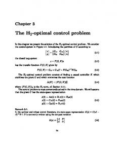
The H2-optimal control problem In this chapter we present the solution of the H -optimal control problem. We consider the control system in Figure 1.2. Introducing the partition of G according to 2
� �
z = �G y G
11 21
the closed-loop system
G G
12
��
22
v� u
(3.1)
z = F (G; K )v
(3.2)
has the transfer function F (G; K ) given by
F (G; K ) = G + G (I , KG ), KG 11
12
22
1
21
(3.3)
The H -optimal control problem consists of nding a causal controller K which stabilizes the plant G and which minimizes the cost function 2
J (K ) = kF (G; K )k
(3.4)
2 2
2
where kF (G; K )k is the H norm, cf. Section 2.2.1. The control problem is most conveniently solved in the time domain. We will assume that the plant G has the state-space representation 2
2
x_ (t) = Ax(t) + B v(t) + B u(t) z(t) = C x(t) + D u(t) y(t) = C x(t) + D v(t) 1
2
1
12
2
21
(3.5)
Remark 3.1.
In the optimal and robust control literature, the state-space representation G(s) = C (sI , A),1 B + D is commonly written using the compact notation �
� A B G(s) := C D
24
(3.6)
Hence the systems in (3.5) can also be written as 2
G(s) := 4
A B B C D D C D D 1
2
1
11
12
2
21
22
3 5
(3.7)
where D11 = 0, D22 = 0.
In (3.5), the direct feedthrough from v to z has been assumed zero in order to obtain a nite H norm for the closed-loop system. The direct feedthrough from u to y has been assumed zero because physical systems always have a zero gain at in nite frequency. It is convenient to make the following assumptions on the system matrices. 2
Assumptions: (A1) The pair (A; B ) is stabilizable. (A2) DT D is invertible. (A3) DT C = 0. (A4) The pair (C ; A) has no unobservable modes on the imaginary axis. (B1) The (C ; A) is detectable. (B2) D DT is invertible. (B3) D B T = 0. (B4) The pair (A; B ) has no uncontrallable modes on the imaginary axis. 2
12
12
12
1
1
2
21
21
21
1
1
The rst set of assumptions (A1){(A4) is related to the state feedback control problem, while the second set of assumptions (B1){(B4) is related to the state estimation problem. Assumptions (A1) and (B1) are necessary for a stabilizing controller u = Ky to exist. Assumptions (A2), (A3) and (B2), (B3) can be relaxed, but they are not very restrictive, and as we will see they imply convenient simpli cations in the solution. Assumptions (A4) and (B4) are required for the Riccati equations which characterize the optimal controller to have stabilizing solutions. These assumptions can be relaxed, but the solution of the optimal control problem must then be characterized in an alternative way, for example in terms of linear matrix inequalities (LMIs). It is appropriate to introduce the time-domain characterization in (2.45) of the cost (3.4), giving m Z1 X J (K ) = [ z(t)T z(t)dt : v = ek �(t)] (3.8) 2
k=1
0
Notice, however, that the characterization (3.8) is introduced solely because the solution of the H -optimal control problem can be derived in a convenient way using (3.8). On the other hand, the motivation of the H -optimal is often more naturally stated in terms of the average frequency-domain characterization in (2.15) or the stochastic characterization in (2.46). 2
2
25
Remark 3.2.
In the linear quadratic optimal control literature, the cost function is usually de ned as
JLQ(K ) =
m �Z X k=1
1
0
[x(t)T Qx(t) + u(t)T Ru(t)]dt : v = e
k �(t)
�
(3.9)
where Q is a symmetric positive semide nite matrix and R is a symmetric positive de nite matrix. It is easy to see that the cost functions (3.8) and (3.9) are equivalent, because the positive (semi)de nite matrices Q and R can always be factorized as
Q = (Q = )T Q = ; R = (R = )T R = 1 2
1 2
1 2
(3.10)
1 2
The factorizations in (3.10) are called Cholesky factorizations, cf. the MATLAB routine chol. De ning the matrices � 1=2 � � � Q 0 C1 = 0 ; D12 = R1=2 (3.11) it follows that
zT z = (C x + D u)T (C x + D u) = xT Qx + uT Ru
(3.12) and the costs (3.8) and (3.9) are thus equivalent. Notice also that with C1 and D12 de ned by (3.11), assumption (A3) holds. 1
12
1
12
The solution of the H -optimal control problem can be done in two stages. In the rst stage, an optimal state-feedback law is constructed. The second stage consists of nding an optimal state estimator. 2
3.1 The optimal state-feedback problem The following result gives the optimal state-feedback law u^(s) = Kx(s)^x(s) which minimizes the quadratic cost (3.8) or (3.9). The result is classical in optimal linear quadratic (LQ) control theory.
Theorem 3.1 H -optimal state feedback control. 2
Consider the system (3.5). Suppose that the assumptions (A1){(A4) hold. Assume that the control signal u(t) has access to the present and past values of the state, x(� ); � � t. Then the cost (3.8) is minimized by the static state state-feedback controller
u(t) = Kopt x(t) where
(3.13)
Kopt = ,(DT D ), B T S
(3.14) and where S is the unique symmetric positive (semi)de nite solution to the algebraic Riccati equation (ARE) 12
1
12
2
AT S + SA , SB (DT D ), B T S + C T C = 0 2
12
12
26
1
2
1
1
(3.15)
such that the matrix
A + B Kopt
(3.16)
2
is stable, i.e. all its eigenvalues have negative real parts. Moreover, the minimum value of the cost (3.8) achieved by the control law (3.13) is given by min J (K ) = tr(B1T SB1 ) (3.17) K 2 x x
By the theory of Riccati equations it follows from assumptions (A1) and (A4) that the algebraic Riccati equation (3.15) has a positive (semi)de nite solution S such that the matrix in (3.16) is stable. Consider the integral in (3.8). It can be decomposed as Proof:
Z
1
0
z(t)T z(t)dt =
Z 0+
Z 1 T z(t) z(t)dt + z(t)T z(t)dt
(3.18)
+
0
0
where 0+ denotes the time immediately after the impulse input at time t = 0. With x(0) = 0 and v(t) = ek �(t), we have formally
x(0 ) = +
Z 0+ 0
eA +,� [B ek �(� ) + B u(� )]d� = B ek (0
)
1
2
(3.19)
1
It follows that the rst integral in (3.18) is zero. Assuming that the algebraic Riccati equation (3.15) has a positive (semi)de nite solution, the second integral in (3.18) can be expanded as Z
1
0+
z(t)T z(t)dt =
Z
1
0+
Z
[C1 x(t) + D12 u(t)]T [C1 x(t) + D12 u(t)]dt
1h
T
[C1 x(t) + D12 u(t)]T [C1 x(t) + D12 u(t)] + d(x(t)dtSx(t)) dt + 0 , x(1)T Sx(1) + x(0+ )T Sx(0+ ) Z 1 T D [u(t) , u0 (t)]dt + x(0+ )T Sx(0+ ) = + [u(t) , u0 (t)]T D12 (3.20) 12 =
i
0
where
u (t) = Kopt x(t);
(3.21) and x(0+ ) denotes the state immediately after the impulse input at time t = 0. We have also assumed that x(1) = 0 due to stability, and used the fact that S satis es (3.15). Introducing (3.20) and (3.19), the cost (3.8) can be expressed as 0
J (K ) = 2
= =
m �Z X
1
k=1 0 m �Z 1 X k=1 0 m �Z 1 X k=1
0
�
z(t)T z(t)dt : v = ek �(t) = [u(t) , u
(t)]T DT D
[u(t) , u
T D12 [u(t) , u0 (t)]dt + eT B T SB1 e (t)]T D12 k k 1
0
0
12
12
[u(t) , u (t)]dt + x(0 0
+
�
)T Sx(0+ ) : v = ek �(t) : v = ek �(t)
�
(3.22) 27
Here
m X eT B T SB
k=1
k
1
1
ek =
m X k=1
tr(B1T SB1 ek eTk ) = tr(B1T SB1
m X
ek eTk ) = tr(B T SB )
(3.23)
1
1
k=1
Hence,
J (K ) = 2
m �Z X k=1
1 0
[u(t) , u
0
(t)]T DT
12
�
D [u(t) , u (t)]dt : v = ek �(t) + tr(B T SB ) (3.24) 0
12
1
1
Since the integrals in (3.24) are non-negative, and are equal to zero when u(t) = u0 (t), it follows that the cost J2 (Kx ) is minimized by the static state feedback (3.13), or (3.21), and the minimum cost is given by (3.17). 2
Problem 3.1. Verify the last step in (3.20). Notice that the optimal state-feedback controller consists of a static state feedback, although no restrictions on the controller structure was imposed. Another point to notice about the optimal controller is that it does not depend on the disturbance v, since the controller is independent of the matrix B1. This matrix enters only in the expression (3.17) for the minimum cost.
Remark 3.3.
By equation (3.20), the control law (3.21) is optimal for all initial states x(0+ ). This implies that the solution of the H2 control problem can be interpreted in a worst-case setting as the controller which minimizes the worst-case cost n
o
J ;worst(K ) := max kzk : xT (0)x(0) � 1 x 2
(0)
= max
2 2
�Z
x(0)
0
� 1 T z (t)z(t)dt : xT (0)x(0) � 1
(3.25)
The optimal state-feedback control result suggests how an optimal output feedback controller u^(s) = K (s)^y(s) can be obtained. In particular, the integral in the expansion (3.22) cannot be made equal to zero if the whole state vector x(t) is not available to the controller. In the output feedback problem, one should instead make this integral as small as possible by using an optimal state estimate x^(t) instead. Therefore, we give next the solution to an H -optimal state estimation problem. 2
3.2 The optimal state-estimation problem In this section we consider the system
x_ (t) = Ax(t) + B v(t) z(t) = C x(t) y(t) = C x(t) + D v(t) 1
1 2
21
28
(3.26)
Notice that in the estimation problem, we need not consider the input u. As u is a known input, its e�ect on the state is exactly known. We consider stable causal state estimators F such that the state estimate x^(t) is determined from the measured output y according to (in the Laplace-domain) x^(s) = F (s)y(s). In the H -optimal estimation problem, the problem is to construct an estimator such that the quadratic H -type cost 2
2
Je(F ) =
m Z X
k=1
[
1 0
[x(t) , x^(t)]T C T C [x(t) , x^(t)]dt : v = ek �(t)] 1
1
(3.27)
is minimized. The solution of the optimal state estimation problem is given as follows.
Theorem 3.2 H -optimal state estimation. 2
Consider the system (3.26). Suppose that the assumptions (B1){(B4) hold. The stable causal state estimator which minimizes the cost (3.27) is given by x^_ (t) = Ax^(t) + L[y(t) , C2x^(t)] (3.28) where L = PC2T (D21 D21T ),1 (3.29) and where P is the unique symmetric positive (semi)de nite solution to the algebraic Riccati equation AP + PAT , PC2T (D21 D21T ),1C2P + B1B1T = 0 (3.30) such that the matrix A , LC2 (3.31) is stable, i.e. all its eigenvalues have negative real parts. Moreover, the minimum value of the cost (3.27) achieved by the estimator (3.28) is given by min J (F ) = tr(C1PC1T ) (3.32) F e
Remark 3.4.
Notice that the optimal state estimator is independent of the matrix C1 in the cost (3.27). The matrix enters only in the expression (3.32) for the minimum cost.
Remark 3.5.
The solution de ned by (3.29) and (3.30) is the dual to the solution (3.14) and (3.15) of the optimal state-feedback problem in the sense that (3.14) and (3.15) reduce to (3.29), (3.30) by making the substitutions
A ! AT C ! BT B ! CT D ! DT 1
1
2
2
12
21
29
(3.33)
and the costs (3.17) and (3.32) are dual under the substitution B1 ! C1T .
The estimator (3.28) is the celebrated Kalman lter due to Rudolf Kalman and R. S. Bucy (1960, 1961). Originally, it has been introduced in a stochastic framework for recursive state estimation in stochastic systems. Notice that the cost (3.27) equals the H norm of the transfer function from the disturbance v to the estimation error C (x , x^). From what was mentioned previously in Section 2.2.1 it follows that if v is stochastic white noise, the cost (3.27) can be characterized as Z tf 1 J (F ) = lim E [ [x(t) , x^(t)]T C C [x(t) , x^(t)]dt] (3.34) 2
1
e
tf
tf !1
1
0
1
Remark 3.6.
In the standard formulation of the stochastic estimation problem the system is de ned as
x_ (t) = Ax(t) + v (t) z(t) = C x(t) y(t) = C x(t) + v (t) 1
(3.35)
1 2
2
where v1 (t) and v2 (t) are mutually independent white noise processes with covariance matrices R1 and R2, respectively. This formulation reduces to the one above by the identi cations � R1 0 � = � B1 � [ B T DT ] (3.36) 0 R2 D21 1 21 and � � � v1 = B1 � v (3.37) v D 2
21
The optimal estimator result is more di�cult to prove than the optimal statefeedback controller. We shall only provide a proof based on duality between the optimal state-feedback and estimation problems. Proof of Theorem 3.2: Consider a state estimator x^(s) = F (s)y with transfer function F (s). Then we have in terms of operators,
C (x , x^) = [C G , C FG ]v 1
1
1
1
(3.38)
2
where (cf. (3.26))
G (s) = (sI , A), B ; G (s) = C (sI , A), B + D 1
1
1
2
1
2
1
21
(3.39)
The cost (3.27) can then be characterized as
Je(F ) = kC G , C FG k (3.40) But by the de nition (2.15), the H norm of a transfer function matrix is equal to the H 1
norm of its transpose. Hence
1
1
2 2 2
2
2
Je(F ) = kGT C T , GT F T C T k 1
1
30
2
1
2 2
(3.41)
Notice that Hence
�
C G (s) � = � C � (sI , A), B + � 0 G (s) C D 1
1
2
1
1
2
1
�
21
T ] [ G1 (s)T C1T G2 (s)T ] = B1T (sI , AT ),1 [ C1T C2T ] + [ 0 D21 and the transposed system � � T T T r = [ G1 C1 G2 ] ��
(3.42) (3.43) (3.44)
thus has the state-space representation p_(t) = AT p(t) + C1T � (t) + C2T �(t) r(t) = B1T p(t) + D21T �(t) (3.45) Using the control law � = ,F T C1T � (3.46) the closed-loop system (3.44), (3.46) is described by r = (GT1 C1T , GT2 F T C1T )� (3.47) Hence the H2 -optimal estimation problem is equal to the dual control problem which consists of nding a controller (3.46) such that the H2 norm of the closed-loop system is minimized. The dual control problem is, however, equivalent to a state-feedback control problem, because the fact that C1T � is available to the controller means that the state p(t) in (3.45) is also available. More speci cally, the problem of nding a control law (3.46) which minimizes the H2 norm of the closed-loop transfer function, equation (3.41), is equivalent to the problem of nding a state-feedback law �(t) = ,FpT p(t) (3.48) where p(t) is available through equation (3.45) and knowledge of C1 � (t) and �(t). But the problem of nding an optimal state-feedback controller for the dual system (3.45) is known, and from our previous result it is given by (3.14) and (3.15) under to the substitutions (3.33). This gives the optimal stationary state-feedback with T p(t); F T = (D DT ),1 C P �(t) = ,Fopt (3.49) 21 2 opt 21 where P is given by the algebraic Riccati equation (3.30). In order to derive the optimal state estimator, notice that combining (3.49) and (3.45), the dual state-feedback controller (3.49) corresponds to a controller � = ,F T C1T � , (3.46), with state-space representation T p(t) p_(t) = AT p(t) + C1T � (t) , C2T Fopt = (A , Fopt C2 )T p(t) + C1T � (t) (3.50) T �(t) = ,Fopt p(t) Taking the negative of the transpose of (3.50) gives the state-space representation of (F T C1T )T = C1F , and thus the optimal estimator x^ = Fy, x^_ (t) = (A , Fopt C2)^x(t) + Fopt y(t) z^(t) = C1x^(t) (3.51) 31
2
which is equal to (3.28).
Remark 3.7.
As noted above, the H2 -optimal estimator is dual to an optimal state feedback problem. It follows that for all the properties of the latter there is a corresponding dual property of the former. In particular, it follows from Remark 3.3 that the optimal estimator can be interpreted as a worst-case estimator as follows. By Remark 3.3 the dual state-feedback problem gives the optimal controller (3.49) which minimizes the worst-case performance from p(0) 2 Rn to r 2 L2 [0; 1). By duality of the optimal estimation and the optimal state feedback problem, it follows that the optimal estimator can be interpreted in a worst-case setting as the estimator which minimizes the worst-case estimation error n o 2 Je;worst(K ) := max k x ( t ) , x ^ ( t ) k : k v k 2 � 1 v = max v
�
[x(t) , x^(t)]T [x(t) , x^(t)] :
Z t
,1
vT (� )v(� )d�
�1
�
(3.52)
This observation gives a nice deterministic interpretation of the Kalman lter as the lter which minimizes the pointwise worst-case estimation error. This property can be compared with the H1 estimator, which will be studied in section 4.2.
3.3 The optimal output feedback problem We are now ready to present the solution to the H -optimal control problem for the system shown in Fig. 1.2. The solution will be based on the cost function expansion in equation (3.24). Recall that (3.24) can be written as 2
J (K ) = 2
m �Z X
k=1
1
0
[u(t) , Kopt
�
x(t)]T DT D 12
12
[u(t) , Kopt x(t)]dt : v = ek �(t)
+tr(B T SB ) (3.53) In contrast to the state-feedback case, when only the output y is available to the controller the integrals cannot be made equal to zero. Instead, the cost (3.53) is equivalent to an H -optimal state estimation problem, because the best one can do is to compute an estimate x^ of the state, and to determine the control signal according to u(t) = Kopt x^(t) (3.54) giving the cost 1
1
2
J (K ) = 2
m �Z X
k=1
1
0
�
T DT D K [^ [^x(t) , x(t)]T Kopt opt x(t) , x(t)]dt : v = ek � (t) 12
12
+tr(B T SB ) (3.55) Hence, it follows that the minimum of the quadratic cost (3.8) is achieved by the controller (3.54), where x^ is an H -optimal state estimate for the system (3.5). We summarize the result as follows. 1
1
2
32
Theorem 3.3 H -optimal control. 2
Consider the system (3.5). Suppose that the assumptions (A1){(A4) and (B1){(B4) hold. Then the controller u = Ky which minimizes the H2 cost (3.8) is given by the equations x^_ (t) = (A + B2 Kopt)^x(t) + L[y(t) , C2 x^(t)] u(t) = Koptx^(t) (3.56) where
Kopt = ,(DT D ), B T S 12
and
1
12
(3.57)
2
L = PC T (D DT ),
(3.58) and S and P are the symmetric positive (semi)de nite solutions of the algebraic Riccati equations (3.15) and (3.30), respectively. Moreover, the minimum value of the cost achieved by the controller (3.56) is 21
2
1
21
T DT ) + tr(B T SB ) min J (K ) = tr(D Kopt PKopt K 2
12
12
(3.59)
1
1
Proof: First we show that the optimal controller (3.56) gives a stable closed loop. Introduce the estimation error x~(t) := x(t) , x^(t). Then the closed loop consisting of the system (3.5) and the controller (3.56) is given by � �
� x_ = � A + B Kopt ,B Kopt � � x � + � B (3.60) x~_ 0 A , LC x~ B , LD v Stability of the closed-loop follows from stability of the matrices A + B Kopt and A , LC . The fact that the controller (3.56) minimizes the H cost (3.8) follows from the expansion (3.53) of Theorem 3.1 and Theorem 3.2. 2 The optimal controller (3.56) consists of an H -optimal state estimator, and an H -optimal state feedback of the estimated state. A particular feature of the solution is that the optimal estimator and state feedback can be calculated independently of each other. This feature of H -optimal controllers is called the separation principle. 2
2
1
2
1
21
2
2
2
2
2
Remark 3.8.
2
The optimal controller (3.56) is a classical result in linear optimal control, where one usually assumes that the disturbances are stochastic white noise processes with a Gaussian distribution (cf. Remark 3.6), and the cost is de ned as # Z tf 1 T T JLQG(K ) = tflim !1 E tf 0 [x(t) Qx(t) + u(t) Ru(t)]dt "
(3.61)
cf. Remark 3.1. This problem is known as the Linear Quadratic Gaussian (LQG) control problem. 33
3.4 Some comments on the application of H2 optimal control The H -optimal (LQG) control problem solves a well-de ned optimal control problem de ned by the quadratic cost in (3.4), (3.8), or (3.61). Practical applications of the method require, however, that the cost be de ned in a manner which corresponds to the control objectives. This is not always very straightforward to achieve, and some observations are therefore in order. Here, we will only discuss two particular problems in H controller design. The rst one concerns the problem of applying the approach to the case with general deterministic inputs, not necessarily impulses. The second problem is concerned with the selection of weights in the quadratic cost (3.61). 2
2
H -optimal control against general deterministic inputs 2
In the deterministic interpretation of the H cost, equation (3.8), it is in many cases not very realistic to assume an impulse disturbance. For example, a step disturbance would often be a more realistic disturbance form. It is therefore important to generalize the control problem to other types of deterministic disturbance signals. Assume that the system (3.5) is subject to an input v with a rational Laplacetransform. Such an input can be characterized in the time domain by a state-space equation x_ v (t) = Av xv (t); x(0) = b v(t) = Cv xv (t) (3.62) or x_ v (t) = Av xv (t) + bw(t); w(t) = �(t) v(t) = Cv xv (t) (3.63) where the input w is an impulse function. By augmenting the system (3.5) with the disturbance model (3.63), the problem has thus been taken to the standard form with an impulse input. One problem with the above approach is that for some important disturbance types, such as step, ramp and sinusoidal disturbances, the disturbance model (3.63) is unstable. As the disturbance dynamics is not a�ected by the controller, the augmented plant consisting of (3.5) and (3.63) will not be stabilizable. It follows that the Riccati equation (3.15) does not have a stabilizable solution in these cases. This problem can be handled in the following way, which we will here demonstrate for the case with a step disturbance. Assume that the disturbance v is a step disturbance, described by � ; t> 0. A more direct approach is, however, to eliminate the unstabilizable mode. This is achieved by di�erentiating the system equations (3.5), giving x(t) = Ax_ (t) + B v_ (t) + B u_ (t) y_ (t) = C x_ (t) + D v_ (t) (3.66) Notice that if the input u is weighted in the cost, a steady-state o�set after the step disturbance will result. Therefore, it is more realistic to weight the input variation u_ (t) instead. The controlled output z is therefore rede ned according to z(t) = C x(t) + D u_ (t) (3.67) Introducing zx := C x, the system can be written as 2 3 2 32 3 2 3 2 3 x ( t ) A 0 0 x _ ( t ) B B 6 7 6 0 0 75 64 zx(t) 75 + 64 0 75 v_ (t) + 64 0 75 u_ (t) 4 z_x (t) 5 = 4 C y_ (t) C 0 02 y(3t) D 0 x_ (t) z(t) = [ 0 I 0 ] 64 zx(t) 75 + D u_ (t) (3.68) y(t) 3 2 x_ (t) 7 6 y(t) = [ 0 0 I ] 4 zx(t) 5 y(t) This characterization is in standard form with an impulse disturbance input v_ given by (3.65). Notice, however, that assumption (B2) associated with the measurement noise does not hold. In order to satisfy this assumption as well, we can add a noise term vmeas on the measured output, 2 3 x _ ( t ) y(t) = [ 0 0 I ] 64 zx(t) 75 + vmeas(t) (3.69) y(t) As there is often a measurement noise present in practical situations, this modi cation seems to be realistic one. 1
2
2
21
1
12
1
1
2
1 2
21
12
Selection of weighting matrices in H -optimal control 2
The second design topic which we will discuss is the speci cation of the controlled output z, or equivalently, the choice of weighting matrices Q and R in the quadratic cost (3.9) or (3.61). For convenience, we will focus the discussion in this section on the stochastic problem formulation, and the associated cost (3.61). It has been stated that the LQG problem is rather arti cial, because the quadratic cost (3.61) seldom, if ever, corresponds to a physically relevant cost in practical applications. This may hold for the quadratic cost (3.61). However, it should be noted that 35
it is often meaningful to consider the variances of the individual variables. Therefore, we introduce the individual costs " Z # tf 1 2 Ji(K ) = tflim !1 E tf 0 xi(t) dt ; i = 1; : : : ; n " Z # tf 1 2 Jn+i(K ) = tflim (3.70) !1 E tf 0 ui(t) dt ; i = 1; : : : ; m Thus, the costs Ji(K ); i = 1; : : : ; n denote the variances of the state variables, and Jn+i(K ) denote the variances of the inputs. In contrast to the quadratic cost (3.61), the individual costs Ji(K ) are often physically relevant. If the states xi represent quality variables (such as concentrations, basis weight etc), then the variance is a measure of the quality variations. The input variances, again, show how much control e�ort is required. It is therefore well motivated to control the system in such a way that all the individual costs (3.70) are as small as possible. As all the costs cannot be made arbitrarily small simultaneously, the problem de ned in this way is a multiobjective optimization problem, and it can be solved e�ciently using techniques developed in multiobjective optimization. The set of optimal points in multiobjective optimization is characterized by the set Pareto-optimal, or noninferior, points. De nition 3.1. (Pareto-optimality) Consider the multiobjective control problem associated with the individual costs Ji(K ), i = 1; : : : ; n + m in equation (3.70). A stabilizing controller K0 is a Pareto-optimal, or noninferior, controller if there exists no other stabilizing controller K such that Ji(K ) � Ji(K0) for all i = 1; : : : ; n + m and Jj (K ) < Jj (K0 ) for some j 2 f1; : : : ; n + mg Thus, a Pareto-optimal controller is simply any controller such that no individual cost can be improved without making at least one other cost worse. It is clear that the search for a suitable controller should be made in the set of Pareto-optimal controllers. The multiobjective optimal control problem is connected to the H2 or LQG optimal control problem as follows. It turns out that the set of Pareto-optimal controllers consists of precisely those controllers which minimize linear combinations of the individual costs, i.e.,
JLQG(K ) =
n X
qiJi(K ) +
i=1"
m X
riJn+i(K ) i=1 # Z tf T T [x(t) Qx(t) + u(t) Ru(t)]dt
= E t1 f 0 where
Q = diag (q1 ; : : : ; qn) ; R = diag (r1; : : : ; rm) 36
(3.71) (3.72)
and qi; ri are positive. The multiobjective control problem is thus reduced to a selection of the weights in the LQ cost in such a way that all the individual costs Ji(K ) have satisfactory values. Thus, although the LQ cost may not be physically well motivated as such, it is still relevant via the individual costs Ji(K ), which often can be motivated physically. There are systematic methods to nd suitable weights (3.72) in such a way that the individual costs have satisfactory values. A particularly simple case is when one cost, Jj (K ) say, is the primary cost to be minimized, while the other costs should be restricted. In this case the problem can be formulated as a constrained minimization problem, Minimize Jj (K ) (3.73) subject to Ji(K ) � c2 ; i = 1; : : : ; n + m; i 6= j (3.74) 3.5
Literature
In addition to the books referenced in Chapter 1, there are some excellent classic texts on the optimal LQ and LQG problems. Standard texts on the subject are for example Anderson and Moore (1971, 1979), � Astrom (1970) and Kwakernaak and Sivan (1970). A newer text with a very extensive treatment of the theory is Grimble and Johnson (1988). The minimax property of the Kalman lter, which was mentioned in Remark 3.7, has been observed by many people, see for example Krener (1980). The multiobjective approach to LQG design described in Section 3.4 has been discussed in Toivonen and Makila (1989).
References
Anderson, B. D. O. and J. B. Moore (1971). Linear Optimal Control. Prentice-Hall, Englewood Cli�s, N.J. Anderson, B. D. O., and J. B. Moore (1971). Optimal Filtering. Prentice-Hall, Englewood Cli�s, N.J. � Astrom, K. J. (1970). Introduction to Linear Stochastic Control Theory. Academic Press, New York. Grimble, M. J. and M. A. Johnson (1988). Optimal Control and Stochastic Estimation. Volumes 1 and 2. Wiley, Chichester. Krener, A. J. (1980). Kalman-Bucy and minimax ltering. IEEE Transactions on Automatic Control Theory AC-25, 291{292. Kwakernaak, H. and R. Sivan (1972). Linear Optimal Control Systems. Wiley, New York. Toivonen, H. T. and P. M. Makila (1989). Computer-aided design procedure for multiobjective LQG control problems. Int. J. Control 49, 655{666. 37