Forecasting Return Volatility of the CSI 300 Index Using the Stochastic

Hindawi Publishing Corporation Discrete Dynamics in Nature and Society Volume 2014, Article ID 964654, 10 pages http://dx.doi.org/10.1155/2014/964654

Research Article Forecasting Return Volatility of the CSI 300 Index Using the Stochastic Volatility Model with Continuous Volatility and Jumps Xu Gong, Zhifang He, Pu Li, and Ning Zhu School of Business, Central South University, Changsha, Hunan 410083, China Correspondence should be addressed to Ning Zhu; [email protected] Received 13 April 2014; Accepted 12 June 2014; Published 9 July 2014 Academic Editor: Chuangxia Huang Copyright © 2014 Xu Gong et al. This is an open access article distributed under the Creative Commons Attribution License, which permits unrestricted use, distribution, and reproduction in any medium, provided the original work is properly cited. The logarithmic realized volatility is divided into the logarithmic continuous sample path variation and the logarithmic discontinuous jump variation on the basis of the SV-RV model in this paper, which constructs the stochastic volatility model with continuous volatility (SV-CJ model). Then, we use high-frequency transaction data for five minutes of the CSI 300 stock index as the study sample, which, respectively, make parameter estimation on the SV, SV-RV, and SV-CJ model. We also comparatively analyze these three models’ prediction accuracy by using the loss functions and SPA test. The results indicate that the prior logarithmic realized volatility and the logarithmic continuous sample path variation can be used to predict the future return volatility in China’s stock market, while the logarithmic discontinuous jump variation is poor at its prediction accuracy. Besides, the SV-CJ model has an obvious advantage over the SV and SV-RV model as to the prediction accuracy of the return volatility, and it is more suitable for the research concerning the problems of financial practice such as the financial risk management.

1. Introduction Recent papers (such as Corsi [1], Wen and Yang [2], Liu et al. [3], Andersen et al. [4, 5], Dai et al. [6], Wen et al. [7], Bollerslev et al. [8, 9], and Liu et al. [10–12]) have showed that the financial risk management, financial asset pricing, and financial derivatives pricing play more and more important roles in the analysis of the problems in financial practices. What is more, the research on the asset volatility of the financial market is the basis of the analysis of the problems in financial practices like the financial risk management, financial asset pricing, and financial derivatives pricing. Therefore, the measurement and forecast of financial asset volatility have become hot topics. In order to accurately measure and predict the financial asset volatility, Engle [13] proposed an ARCH model according to “clustering” and “long-memory” features of the return volatility; Bollerslev [14], on the basis of the ARCH model, established a GARCH model. Taylor [15] first proposed a stochastic volatility (SV) model. Then, many scholars study the SV model and comparatively analyze the measurement

and forecast accuracy for financial asset volatility between the GARCH model and SV model. Among them, there are many literatures about the comparison of SV model and GARCH model on asset volatility measurement and sample fitting ability. Danielsson [16] studied the S&P 500 index of American stock markets, and he found that the fitting ability of SV model for the S&P 500 index volatility is stronger than the ARCH (5), GARCH (1, 2), IGARCH, and EGARCH (2, 1) model. Wang et al. [17], the empirical study on the application of China’s stock market data, found that the SV model can better describe the heteroscedasticity in the return of stock market and the serial correlation of volatility than GARCH model. Kim et al. [18] also found that the SV model have a better sample fitting ability for the financial asset volatility than the GARCH model. In addition, there exist some literatures about the prediction accuracy of the future financial asset volatility as to the comparative study on SV model and GARCH model. Yu [19], the comparative study on the SV model and GARCH model, found that the SV model showed much better out-of-sample forecasting performance

2

Discrete Dynamics in Nature and Society

than the ARCH and GARCH (1, 1) and GARCH (3, 2) model in New Zealand stock market. Sadorsky [20] (in the US stock market), Pederzoli [21] (in the UK stock market), and Wei [22] (in the crude oil futures market) came to a similar conclusion with Yu [19], that is to say, the SV model’s prediction accuracy is stronger than the GARCH model’s. Although the SV model has good forecasting performance for the future return volatility, higher accuracy is more favorable to the analysis of practical financial problems such as financial risk measuring, financial asset pricing, and financial derivatives pricing. In order to improve the prediction and measurement accuracy of the model, Koopman et al. [23] introduced realized volatility (RV; Andersen and Bollerslev [24]) as an exogenous variable into the volatility equation of SV model so as to construct the SV-RV model. After applying the S&P 100 index in American stock markets, Koopman et al. found the measuring and forecasting accuracy for return volatility of SV-RV model is stronger than the SV model. Then, Geweke et al. [25] found that the SV-RV model has a good ability to predict financial asset volatility. Jacquier and Miller [26] also found that the realized volatility (RV) contained certain prediction information for the future volatility, and the SV-RV model’s prediction ability is superior to the SV model. However, in the real financial market, because of the impact of the abnormal information and the existence of the irrational investors, the financial asset volatility is not only a continuous process but also there are some jumps in it. Therefore, while we study the SV-RV model, it is more reasonable to divide the RV into the continuous sample path variation (C) and the discontinuous jump variation (J) and add the two factors into the volatility equation of SV model. Hence, after learning from Barndorff-Nielsen and Shephard [27, 28] and Andersen et al. [5], on the basis of the SV-RV model, we divide the RV into C and J and establish the SV-CJ model so as to further improve the model’s ability to measure and forecast financial asset volatility. Then, we use the highfrequency data for five minutes of CSI 300 index in China’s stock market as the research sample to make parameter estimation on the SV, SV-RV, and SV-CJ model, respectively, and use the loss functions and SPA test proposed by Hansen [29] to comparatively analyze forecasting performance for the future return volatility of the three models. By this way, we look for the best model for forecasting financial asset volatility. The remainder of this paper is organized as follows. In Section 2, we discuss three volatility models, the SV, SVRV, and SV-CJ model. In Section 3, we introduce estimation and evaluation method of the models. In Section 4, the estimating and forecasting results are presented. Section 5 is the conclusion of this paper.

2. Volatility Models 2.1. The SV and SV-RV Model. In the existing literature, there exist many forms about the SV model; one of the common forms can be expressed as follows: 𝑦𝑡 = 𝜀𝑡 𝑒ℎ𝑡 /2 , ℎ𝑡 = 𝛼 + 𝛽ℎ𝑡−1 + 𝜂𝑡 ,

(1)

where 𝑦𝑡 is a return. {𝜀𝑡 } and {𝜂𝑡 } are mutual dependent. In this paper, we suppose 𝜀𝑡 ∼ 𝑖.𝑖.𝑁(0, 1), 𝜂𝑡 ∼ 𝑖.𝑖.𝑁(0, 𝜎𝜂2 ), and 𝜎𝜂2 is unknown. 𝛼 and 𝛽 are constant. 𝛽, as continuous parameter, reflects the impact of the prior volatility on the current volatility, and when |𝛽| < 1, it stands for covariance stationary of the SV model. ℎ𝑡 is the logarithm of return volatility; supposing ℎ0 ∼ 𝑁(𝛼, 𝜎𝜀2 ), we can conclude that for given ℎ𝑡−1 , 𝛼, 𝛽, ℎ𝑡 obeys normal distribution with mean 𝛼 + 𝛽ℎ𝑡−1 and variance 𝜎𝜀2 ; that, is ℎ𝑡 | ℎ𝑡−1 , 𝛼, 𝛽 ∼ 𝑁(𝛼 + 𝛽ℎ𝑡−1 , 𝜎𝜀2 ), 𝑡 = 1, 2, . . . , 𝑇. To enhance the model’s accuracy for volatility measurement and prediction, according to Koopman et al. [23], we add ln(RV𝑡−1 ) as an exogenous variable to the volatility equation of SV model; we establish the SV-RV model 𝑦𝑡 = 𝜀𝑡 𝑒ℎ𝑡 /2 , ℎ𝑡 = 𝛼 + 𝛽ℎ𝑡−1 + 𝛾 ln (RV𝑡−1 ) + 𝜂𝑡 ,

(2)

where RV𝑡−1 is a realized volatility at time 𝑡 − 1; the volatility used in this paper is identical to that in Martens [30] and Koopman et al. [23]; taking the overnight return variance into consideration, RV𝑡−1 can be expressed as follows: 𝑁

𝑀

𝑖=1

𝑗=1

2 2 2 + 𝑟𝑡,𝑛 = ∑𝑟𝑡,𝑗 , RV𝑡 = ∑𝑟𝑡,𝑗

𝑀 = 𝑁 + 1,

(3)

where 𝑟𝑡,1 and 𝑟𝑡,𝑛 stand for the overnight return, 𝑟𝑡,1 = 𝑟𝑡,𝑛 = 100(ln 𝑃𝑡,𝑜 − ln 𝑃𝑡−1,𝑐 ), 𝑃𝑡,𝑜 represents the open price at time 𝑡, and 𝑃𝑡−1,𝑐 denotes the closing price of phase 𝑡 − 1; 𝑟𝑡,2 is the 1st return after the opening of time 𝑡, 𝑟𝑡,2 = 100(ln 𝑃𝑡,1 − ln 𝑃𝑡,𝑜 ); 𝑃𝑡,1 is the 1st close price after the opening of time 𝑡; 𝑟𝑡,3 shows the 2nd return after the opening of time 𝑡, 𝑟𝑡,3 = 100(ln 𝑃𝑡,2 − ln 𝑃𝑡,1 );. . .; 𝑟𝑡,𝑀 is the (𝑀 − 1)th return after the opening of time 𝑡, and 𝑟𝑡,𝑀 = 100(ln 𝑃𝑡,𝑀−1 − ln 𝑃𝑡,𝑀−2 ). 2.2. The SV-CJ Model. In the real financial market, since the impact of information and irrational behavior of investors, the volatility of return on asset is no longer continuous,while there are some jumps. Andersen et al. [31] have shown that the separation of the realized volatility into the continuous sample path variation and the discontinuous jump variation will enhance the accuracy to predict future volatility. Therefore, in order to further improve the accuracy to predict the future volatility of the model, we transform the logarithmic realized volatility ln(RV𝑡 ) of model (2) to the logarithmic continuous sample path variation ln(𝐶𝑡 ) and the discontinuous jump variation ln(𝐽𝑡 + 1). When the realized volatility is divided into the continuous sample path variation and the discontinuous jump variation, we need to understand several important concepts. Please assume that return on assets is a continuous process; when we use the quadratic variation (quadratic variation, QV) to describe the total variation of the return volatility on financial assets and the integrated variation (IV) to depict the continuous part of the total variation, we can conclude that the difference between quadratic variation and integrated variation is the jump variation. In fact, the observed

Discrete Dynamics in Nature and Society

3

data are discrete, when they are used by the scholars to estimate the quadratic variation and integrated variation; the realized volatility and realized bipower variation (RBV) can be renamed. Barndorff-Nielsen and Shephard [27, 28] used the quadratic variation theory to separate realized volatility into the continuous sample path variation and the discontinuous jump variation. A mathematical description of this decomposition approach is given as follows. Let 𝑝𝑡 = ln(𝑃𝑡 ) denote a logarithmic financial asset price at time 𝑡. The continuous-time jump diffusion process traditionally used in financial asset pricing is conveniently expressed in stochastic differential equation form as 𝑑𝑝𝑡 = 𝜇𝑡 𝑑𝑡 + 𝜎𝑡 𝑑𝑊𝑡 + 𝜅𝑡 𝑑𝑞𝑡 ,

0 ≤ 𝑡 ≤ 𝑇,

(4)

where 𝜇𝑡 is a continuous and locally bounded variation process. 𝜎𝑡 is a strictly positive stochastic volatility process with a sample path that is right continuous and has welldefined left limits (allowing for occasional jumps in volatility). 𝑊𝑡 is a standard Brownian motion. 𝜅𝑡 refers to the size of the corresponding discrete jumps in the logarithmic price process. 𝑞𝑡 represents Poisson counting process of 𝜆 𝑡 , and 𝜆 𝑡 is a time-varying intensity variable, so 𝑃(𝑑𝑞𝑡 = 1) = 𝜆 𝑡 𝑑𝑡. For discrete prices from a continuous time process, the logarithmic return volatility at time 𝑡 is a compound volatility including jump volatility rather than an unbiased estimator of integrated volatility. The log return rate from 𝑡 − 1 to 𝑡 is quadratic variation: QV𝑡 = [𝑟, 𝑟]𝑡 = ∫

𝑡

𝑡−1

𝜎𝑠2 𝑑𝑠 + ∑ 𝜅𝑠2 , 𝑡−1 −𝐴 𝑘 ) , in that,

1 ̂𝑘𝑘 . 𝐴 𝑘 = 𝑛−1/4 𝑤 4

(27)

𝐼{⋅} is an indicator function; as the conditions of the {⋅}, 𝐼{⋅} is 1, otherwise is 0. In the end, we can get the new 𝑇𝑖 statistical magnitude: 𝑖

𝑇𝑖 = max

√𝑛𝑍𝑘 , ̂𝑘𝑘 𝑤

𝑖 = 1, 2, . . . , 𝐵.

(28)

6

Discrete Dynamics in Nature and Society

Hansen [29] showed that under the null hypothesis in (23), formula (28) 𝑇𝑖 statistical magnitude converges to formula (24), as defined by the 𝑇 statistic. Therefore, the 𝑃 values can be obtained directly from the type 𝑖=𝐵

𝑃 = 𝐵−1 ∑𝐼 {𝑇𝑖 > 𝑇} .

(29)

𝑖=1

When comparing the quality prediction model and the test of SPA (the closer to 1), if the 𝑃 value is greater, we cannot refuse the null hypothesis of formula (27) any more. That is to say, compared with other models, the accuracy of the baseline model is much higher.

4. Empirical Evidence 4.1. Data and Summary Statistics. This paper uses the CSI 300 index in China’s stock market to empirical evidence. The data derived from the WIND financial database. The time span of samples is April 20, 2007, to April 20, 2012, and is a total of 1199 days. In the calculation of realized volatility, the daily sample data extracting frequency greatly affects the result of the study. On the one hand, the lower sampling frequency cannot describe the wave information well. On the other hand, the higher sampling frequency will produce micronoise that influenced the results. Therefore, this paper, based on the research of previous scholars (such as Andersen et al. [4, 31] and Huang and Tauchen [32], Huang et al. [33]) and the influence of both hands, uses the CSI 300 index of 5 minutes high frequency data. After eliminating the trading time related data and supplementing the missing data using moving average interpolation method, there are 58751 data, that is, 49 data everyday. (including 1 overnight trading data and 48 intraday trading data). In this paper, we need to use the variables; the rate of return 𝑅𝑡 , the logarithmic realized volatility ln(RV𝑡 ), the logarithmic continuous sample path variation ln(𝐶𝑡 ), and the logarithmic discontinuous jump variation ln(𝐽𝑡 + 1) are all obtained by Matlab 2013a or Excel 2007. Table 1 is descriptive statistics results of 𝑅𝑡 , ln(RV𝑡 ), ln(𝐶𝑡 ), and ln(𝐽𝑡 + 1). From Table 1, we can find that ln(RV𝑡 ) sequence shows the phenomenon of “High Kurtosis and Fat Tail” and does not obey the normal distribution; this shows that China’s stock market volatility is large. In addition, the unit root test (ADF test) shows that every sequence in the 99% confidence interval significantly declined to unit root of null hypothesis, so each sequence is stationary, and we can further analyze the models. 4.2. Parameter Estimation. In Section 2, we introduce Bayesian estimation results of the SV, SV-RV, and SV-CJ model using the MCMC methods through the OpenBUGS software. In order to ensure the convergence of the estimated parameters, 50000 iterations are performed on each parameter in the process of Gibbs sampling; by observing the orbit of the parameters iterations and the autocorrelation function, we found that after 10,000 iterations, the iterative process has converged. Hence, we anneal by using the first

10,000 samples and estimate the model by using the last 40,000 samples in this paper. Table 2 lists the results of the Bayesian parameter estimation of the SV, SV-RV, and SV-CJ model, including the mean, standard deviation, MC error (the error of Monte Carlo simulation value), 95% confidence interval for the posterior, the median, and the value of the deviation information criterion (DIC) of the parameter estimation. Firstly, we analyze the results of Bayesian estimation of the SV and SV-RV model. The estimation value of the parameter 𝛽 is close to 1, explaining that there is a strong persistence and autocorrelation with the return volatility of China’s stock market, in accord with mature capital markets (such as the US and UK) and emerging capital markets (such as South Korea and New Zealand). If the standard deviation and MC error of the parameter are small, the accuracy of the parameter estimation is much higher. In the SV-RV model, estimation of parameter 𝛾 is positive; its standard deviation and MC errors are relatively small and 95% confidence interval for the posterior does not contain the value 0, which proves that the prior logarithmic realized volatility ln(RV𝑡−1 ) has a significant impact on the current volatility. ln(RV𝑡−1 ) contains certain volatility forecast information. Comparing the DIC of SV model and SV-RV model, we find that the DIC of SV-RV model is smaller than that of SV model, which shows that the SV-RV model has a better measuring accuracy to the volatility and agrees with the research results of Koopman et al. [23] and Jacquier and Miller [26]. We focus on the estimation results of SV-CJ model; the coefficient 𝜆 of the logarithmic continuous sample path variation ln(𝐶𝑡−1 ) in the model is positive; its standard deviation and MC errors are relatively small and 95% confidence interval for the posterior does not contain the value 0, which proves that the prior logarithmic continuous sample path variation ln(𝐶𝑡−1 ) has a certain prediction on the current volatility. However, the coefficient 𝜃 of the logarithmic discontinuous jump variation ln(𝐽𝑡−1 + 1) in the model is comparatively large and 95% confidence interval for the posterior contains the value 0, proving that the previous logarithmic discontinuous jump variation ln(𝐽𝑡−1 + 1) has little effect on the current volatility. In addition, comparing the DIC of the models, we can find that the DIC of SV-CJ model is smaller than that of the SV-RV model, which shows that the SV-CJ model has a better measuring accuracy to the volatility and shows that adding the decomposition of the logarithmic realized volatility to the volatility equation SV model can improve the measurement capability to the return volatility. Therefore, when measuring the return volatility, it is more reasonable to use the SV-CJ, SV and SV-RV model.

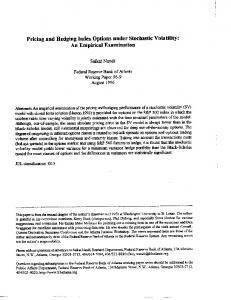
4.3. Forecasting 4.3.1. In-Sample Forecasts. Figure 1 contains a real volatility sequence and three in-sample forecast volatility sequences that are obtained by the SV, SV-RV, and SV-CJ model. To comparatively analyze the predictive accuracy for future volatility of the SV, SV-RV, and SV-CJ model, we use the loss functions and SPA test to compare the predictive accuracy of

Discrete Dynamics in Nature and Society

7 Table 1: Descriptive statistics for each variable.

𝑅𝑡 ln(RV𝑡 ) ln(𝐶𝑡 ) ln(𝐽𝑡 + 1)

∗∗∗

Mean −0.0152 0.9600 0.7650 0.2825

Std. dev. 2.1141 0.9323 0.8992 0.6209

Skewness −0.2647 0.5180 0.3525 3.0445

Kurtosis 4.9345 3.2163 2.8382 14.085

Jarque-Bera 200.95∗∗∗ 55.961∗∗∗ 26.138∗∗∗ 7990.6∗∗∗

ADF-t statistic −32.901∗∗∗ −4.9183∗∗∗ −5.3556∗∗∗ −16.266∗∗∗

Indicates significance at the 1% level.

Table 2: The estimation results of the SV, SV-RV, and SV-CJ model.

SV

SV-RV

SV-CJ

Parameter 𝛼 𝛽 𝛼 𝛽 𝛾 𝛼 𝛽 𝜆 𝜃

Mean 0.0377 0.9694 0.2053 0.6063 0.2870 0.2927 0.5206 0.3566 0.0389

Standard deviation 0.0178 0.0141 0.0594 0.0886 0.0587 0.06966 0.08546 0.05807 0.04991

MC error 0.0011 0.0009 0.0037 0.0057 0.0037 0.0046 0.0059 0.0038 0.0030

these three models in this paper. Table 3 lists the statistical results of the loss functions (the MAE, HMAE, MSE, HMSE, QLIKE, and 𝑅2 LOG) about the SV, SV-RV, and SV-CJ model in the in-sample forecasts. Table 4 lists the SPA test results of SV, SV-RV, and SV-CJ model in the sample in the in-sample forecasts. In Table 3, comparing the size of the loss functions, we find that apart from one point that the QLIKE of SV-RV model is slightly smaller than that of SV-CJ model, the other loss functions of SV model are greater than those of SV-RV model, and the loss functions of SV-RV model are greater than the loss functions of SV-CJ model. In Table 4, the first column represents the baseline model 𝑀0 . Numerical values in the table are the 𝑃 value of SPA test; the larger the 𝑃 value, the stronger the predictive accuracy of the baseline model 𝑀0 , compared with the other two comparison models. In this table, there are four 𝑃 values of SPA test treating the SV-CJ model as a baseline model larger than those of SV-RV model. Similarly, there are four 𝑃 values of SPA test treating SV-RV model as a baseline model larger than those of SV model. Analyzing the results of the loss functions in Table 3 and the results of SPA test in Table 4, we can get the following conclusions. The in-sample forecast accuracy of SV model for return volatility is weaker than that of SV-RV model, and the in-sample forecast ability of SV or SV-RV model for return volatility is weaker than that of SV-CJ model. 4.3.2. Out-of-Sample Forecasts. Compared with the insample predictive accuracy of the model, we are more concerned with the out-of-sample forecasting accuracy, because the out-of-sample forecasting is more meaningful to financial practical issues like the financial risk management, financial asset pricing, financial derivatives pricing, and so on. In order to effectively evaluate the out-of-sample forecasting accuracy

2.5% quantile 0.0136 0.9356 0.1085 0.4152 0.1855 0.1665 0.3548 0.2208 −0.06129

Median 0.0347 0.9860 0.1982 0.6175 0.2823 0.2865 0.5149 0.3623 0.03955

97.5% quantile 0.0798 0.9894 0.3381 0.7541 0.4132 0.4581 0.7192 0.4602 0.1409

DIC 4961.0

4951.0

4938.0

5 4 3 2 1 0 −1 −2

0 50 100 150 200 250 300 350 400 450 500 550 600 650 700 750 800 850 900 950 1000 1050 1100 1150

Model

RV SV

SV-RV SV-CJ

Figure 1: Comparison of the in-sample forecasting performance of the SV, SV-RV, and SV-CJ model. In the figure, RV represents the true volatility; SV, SV-RV, and SV-CJ represent the forecast volatility of the SV, SV-RV, and SV-CJ model, respectively.

of the models, we use the rolling time windows method to test the volatility forecasting accuracy of the SV, SV-RV, and SVCJ model. We select 999 samples as the fixed time windows and the last 200 samples (May 31, 2011–April 20, 2012) as the prediction and evaluation interval. Figure 2 contains a real volatility sequence and three out-of-sample forecast volatility sequences that are obtained by the SV, SV-RV, and SV-CJ model. The analysis approach is consistent with the in-sample forecasting part, still using the loss functions and SPA test to compare the predicting accuracy of each model. The results are shown in Tables 5 and 6. In Table 5, comparing the loss functions, in these three models, apart from one point that the MSE of SV-CJ model is slightly larger than that of SV Model, the other loss functions of SV-CJ are smaller than those of SV and SV-RV model, and the loss functions of SV-RV model are greater than those of SV-CJ model. In addition, comparing the loss functions about the SV and SV-RV models, the loss

8

Discrete Dynamics in Nature and Society Table 3: The loss functions of in-sample forecasts.

SV SV-RV SV-CJ

MAE 2.3879 2.3197 2.2951

HMAE 0.7237 0.7104 0.6736

MSE 1.0140 0.9862 0.8440

HMSE 34.830 32.099 31.167

QLIKE 2.2034 2.1941 2.1983

𝑅2 LOG 0.4572 0.4377 0.4203

QLIKE 0.1882 0.3784 0.7220

𝑅2 LOG 0.7944 0.5798 0.2504

The bold part is the minimum value of each loss function.

Table 4: The SPA test results of in-sample forecasts.

SV SV-RV SV-CJ

MAE 0.0780 0.0408 0.5816

HMAE 0.2056 0.8562 0.5456

MSE 0.1330 0.1382 0.6730

HMSE 0.0538 0.0648 0.6412

Numerical values in the table represent 𝑃 value of SPA test obtained by 5000 Bootstrap simulation; the larger the 𝑃 value, the stronger the in-sample predictive accuracy of the baseline model, compared with the other two comparison models. The bold part is the maximum 𝑃 value of each model’s SPA test.

Table 5: The loss functions of out-of-sample forecasts.

SV SV-RV SV-CJ

MAE 1.3145 1.4186 1.2636

HMAE 1.9953 3.1494 1.4354

MSE 1.0463 1.1515 0.8932

HMSE 7.0803 8.2392 7.6884

QLIKE 1.4152 1.4127 1.3878

𝑅2 LOG 0.6488 0.7103 0.5871

QLIKE 0.0616 0.2538 0.8862

𝑅2 LOG 0.1048 0.0092 0.5442

The bold part is the minimum value of each loss function.

Table 6: The SPA test results of out-of-sample forecasts.

SV SV-RV SV-CJ

MAE 0.2324 0.0262 0.7720

HMAE 0.0300 0.0106 0.6616

MSE 0.0256 0.0248 0.7970

HMSE 0.8558 0.0386 0.0208

Numerical values in the table represent the 𝑃 values of SPA test obtained by 5000 Bootstrap simulation; the larger the 𝑃 value, the stronger out-of-sample predictive accuracy of the baseline model, compared with the other two comparison models. The bold part is the maximum 𝑃 value of each model’s SPA test.

functions of SV model are smaller than those of the SV-RV model apart from the HMSE value. In Table 6, there are five 𝑃 values of SPA test treating SV-CJ model as a baseline model larger than those of SV-RV model and five 𝑃 values of SPA test treating SV model as a baseline model larger than those of SV-RV model. Analyzing the results of loss functions in Table 5 and the results of SPA test in Table 6, we can get the following conclusions. The out-of-sample forecasting accuracy of SVCJ model for return volatility is stronger than that of SV or SV-RV model. The out-of-sample forecast ability of SV model return volatility is stronger than that of SV-RV model. All in all, by analyzing Sections 4.3.1 and 4.3.2, we know that the predictive accuracy for future volatility of SV-CJ model is the strongest in the above three volatility models. Therefore, adding the logarithmic realized volatility ln(RV𝑡−1 ) to the SV volatility model and decomposing ln(RV𝑡−1 ) into the logarithmic continuous sample path variation ln(𝐶𝑡−1 ) and the logarithmic discontinuous jump variation ln(𝐽𝑡−1 + 1), we can improve the model’s performance to predict future volatility. Therefore, this decomposition is meaningful.

5. Conclusion In this paper, we first construct the SV-CJ model based on SV-RV model. Then, we estimate the parameters of SV, SVRV, and SV-CJ models through MCMC methods, using the 5 minutes frequency data in CSI 300 Index of China’s stock market. Finally, using the loss functions and SPA test analyzes the return volatility forecasting accuracy of each model both in-sample and out-of-sample. According to the parameter estimation results of the models, we find that the measuring accuracy for Chinese stock market volatility of SV-CJ model is significantly stronger than that of SV or SV-RV model. The prior logarithmic realized volatility and the prior logarithmic continuous sample path variation contain much predictive information on future volatility while the logarithmic discontinuous jump variation contains little predictive information. Moreover, comparative analysis of the predictive accuracy about the three models indicates that the in-sample forecasting accuracy for return volatility of SV-RV model is stronger than that of SV model. This conclusion may be different from the results of Koopman et al. [23], Jacquier and Miller [26]. It

Discrete Dynamics in Nature and Society 40 35 30 25 20 15 10 5 0

9

[4]

[5] 0

20

40

60

80

RV SV

100

120

140

160

180

200

SV-RV SV-CJ

Figure 2: Comparison of the out-of-sample forecasting performance of the SV, SV-RV, and SV-CJ model. In the figure, RV represents the true volatility; SV, SV-RV, and SV-CJ represent the forecast volatility of the SV, SV-RV, and SV-CJ model, respectively.

may be due to the inconsistency with the model predictive accuracy of future volatility in different markets. In the Chinese stock market, the performance of SV-RV model added RV as the exogenous variables to predict the stock volatility are not significantly stronger than the SV model. However, the volatility forecasting accuracy of SV-CJ model is significantly stronger than the other two models, which shows that using SV-CJ model to measure and predict the volatility is more reasonable in financial practical issues like the financial risk management, financial asset pricing, and financial derivatives pricing. While the SV-CJ model has a better accuracy on volatility measuring and forecasting, it is still necessary to improve the measuring precision and forecasting precision of the volatility model. Therefore, we will further focus on the study to improve the measuring accuracy and forecasting accuracy of the volatility models on the basis of SV-CJ model.

[6]

[7]

[8]

[9]

[10]

[11]

[12]

[13]

[14]

[15]

Conflict of Interests The authors declare that there is no conflict of interests regarding the publication of this paper.

[16]

[17]

Acknowledgment This work was supported in part by the Natural Science Foundation of China (no. 71171024, no. 71371195, and no. 71221061).

References [1] F. Corsi, “A simple approximate long-memory model of realized volatility,” Journal of Financial Econometrics, vol. 7, no. 2, pp. 174–196, 2009. [2] F. Wen and X. Yang, “Skewness of return distribution and coefficient of risk premium,” Journal of Systems Science & Complexity, vol. 22, no. 3, pp. 360–371, 2009. [3] J. Liu, C. Ma, and F. Wen, “An Actuarial approach to option pricing under O-U process and stochastic interest rates,” in Proceedings of the International Joint Conference on Computational

[18]

[19] [20]

[21]

[22]

Sciences and Optimization (CSO ’09), pp. 549–553, IEEE, Sanya, China, April 2009. T. G. Andersen, T. Bollerslev, and X. Huang, “A reduced form framework for modeling volatility of speculative prices based on realized variation measures,” Journal of Econometrics, vol. 160, no. 1, pp. 176–189, 2011. T. G. Andersen, D. Dobrev, and E. Schaumburg, “Jump-robust volatility estimation using nearest neighbor truncation,” Journal of Econometrics, vol. 169, no. 1, pp. 75–93, 2012. Z. Dai, D. Li, and F. Wen, “Robust conditional value-atrisk optimization for asymmetrically distributed asset returns,” Pacific Journal of Optimization, vol. 8, no. 3, pp. 429–445, 2012. F. Wen, Z. Li, C. Xie, and D. Shaw, “Study on the fractal and chaotic features of the Shanghai composite index,” Fractals, vol. 20, no. 2, pp. 133–140, 2012. T. Bollerslev, D. Osterrieder, N. Sizova, and G. Tauchen, “Risk and return: long-run relations, fractional cointegration, and return predictability,” Journal of Financial Economics, vol. 108, no. 2, pp. 409–424, 2013. T. Bollerslev, V. Todorov, and S. Z. Li, “Jump tails, extreme dependencies, and the distribution of stock returns,” Journal of Econometrics, vol. 172, no. 2, pp. 307–324, 2013. J. Liu, L. Yan, and C. Ma, “Pricing options and convertible bonds based on an actuarial approach,” Mathematical Problems in Engineering, vol. 2013, Article ID 676148, 9 pages, 2013. J. Liu, M. Tao, C. Ma, and F. Wen, “Utility indifference pricing of convertible bonds,” International Journal of Information Technology & Decision Making, vol. 13, no. 2, pp. 429–444, 2014. J. Liu, J. Xiao, L. Yan, and F. Wen, “Valuing catastrophe bonds involving credit risks,” Mathematical Problems in Engineering, vol. 2014, Article ID 563086, 6 pages, 2014. R. F. Engle, “Autoregressive conditional heteroscedasticity with estimates of the variance of United Kingdom inflation,” Econometrica, vol. 50, no. 4, pp. 987–1007, 1982. T. Bollerslev, “Generalized autoregressive conditional heteroskedasticity,” Journal of Econometrics, vol. 31, no. 3, pp. 307– 327, 1986. J. S. Taylor, Modeling Financial Time Series, John Wiley & Sons, Chichester, UK, 1986. J. Danielsson, “Stochastic volatility in asset prices estimation with simulated maximum likelihood,” Journal of Econometrics, vol. 64, no. 1-2, pp. 375–400, 1994. F. C. Wang, L. X. Jiang, and G. Li, “Estimating volatility of Chinese stock market by stochastic volatility model,” Journal of Management Sciences in China, vol. 4, pp. 63–72, 2003. S. Kim, N. Shephard, and S. Chib, “Stochastic volatility: likelihood inference and comparison with ARCH models,” Review of Economic Studies, vol. 65, no. 3, pp. 361–393, 1998. J. Yu, “Forecasting volatility in the New Zealand stock market,” Applied Financial Economics, vol. 12, no. 3, pp. 193–202, 2002. P. Sadorsky, “A comparison of some alternative volatility forecasting models for risk management,” in Proceedings of the 2nd IASTED International Conference: Financial Engineering and Applications, 2004. C. Pederzoli, “Stochastic volatility and GARCH: a comparison based on UK stock data,” The European Journal of Finance, vol. 12, no. 1, pp. 41–59, 2006. Y. Wei, “Forecasting volatility of fuel oil futures in China: GARCH-type, SV or realized volatility models?” Physica A: Statistical Mechanics and its Applications, vol. 391, no. 22, pp. 5546–5556, 2012.

10 [23] S. J. Koopman, B. Jungbacker, and E. Hol, “Forecasting daily variability of the S&P 100 stock index using historical, realised and implied volatility measurements,” Journal of Empirical Finance, vol. 12, no. 3, pp. 445–475, 2005. [24] T. G. Andersen and T. Bollerslev, “Answering the critics: yes, ARCH models do provide good volatility forecasts,” International Economic Review, vol. 4, pp. 885–905, 1998. [25] J. Geweke, G. Koop, and H. Dijk, The Oxford Handbook of Bayesian Econometrics, Oxford University Press, 2011. [26] E. Jacquier and S. Miller, “The information content of realized volatility,” Working Paper, HEC Montreal, 2013. [27] O. E. Barndorff-Nielsen and N. Shephard, “Power and bipower variation with stochastic volatility and jumps,” Journal of Financial Econometrics, vol. 2, pp. 1–37, 2004. [28] O. E. Barndorff-Nielsen and N. Shephard, “Econometrics of testing for jumps in financial economics using bipower variation,” Journal of Financial Econometrics, vol. 4, pp. 1–30, 2006. [29] P. R. Hansen, “A test for superior predictive ability,” Journal of Business & Economic Statistics, vol. 23, no. 4, pp. 365–380, 2005. [30] M. Martens, “Measuring and forecasting S&P 500 indexfutures volatility using high-frequency data,” Journal of Futures Markets, vol. 22, no. 6, pp. 497–518, 2002. [31] T. G. Andersen, T. Bollerslev, and F. X. Diebold, “Roughing it up: including jump components in the measurement, modeling, and forecasting of return volatility,” The Review of Economics and Statistics, vol. 89, no. 4, pp. 701–720, 2007. [32] X. Huang and G. Tauchen, “The relative contribution of jumps to total price variance,” Journal of Financial Econometrics, vol. 3, no. 4, pp. 456–499, 2005. [33] C. Huang, X. Gong, X. Chen, and F. Wen, “Measuring and forecasting volatility in Chinese stock market using HAR-CJM model,” Abstract and Applied Analysis, vol. 2013, Article ID 143194, 13 pages, 2013. [34] E. Ruiz, “Quasi-maximum likelihood estimation of stochastic volatility models,” Journal of Econometrics, vol. 63, no. 1, pp. 289–306, 1994. [35] E. Jacquier, N. G. Polson, and P. E. Rossi, “Bayesian analysis of stochastic volatility models,” Journal of Business and Economic Statistics, vol. 12, no. 4, pp. 371–417, 1994. [36] T. G. Andersen and B. E. Sørensen, “GMM estimation of a stochastic volatility model: a Monte Carlo study,” Journal of Business and Economic Statistics, vol. 14, no. 3, pp. 328–352, 1996. [37] T. Watanabe, “A non-linear filtering approach to stochastic volatility models with an application to daily stock returns,” Journal of Applied Econometrics, vol. 14, no. 2, pp. 101–121, 1999. [38] J. Durbin and S. J. Koopman, Time Series Analysis by State Space Methods, vol. 38, Oxford University Press, Oxford, UK, 2nd edition, 2012. [39] L. Bauwens and M. Lubrano, “Bayesian inference on GARCH models using Gibbs sampler,” Econometrics Journal, vol. 1, pp. 23–46, 1998. [40] D. J. Spiegelhalter, N. G. Best, B. P. Carlin, and A. van der Linde, “Bayesian measures of model complexity and fit,” Journal of the Royal Statistical Society B, vol. 64, no. 4, pp. 583–639, 2002. [41] A. P. Dempster, “The direct use of likelihood for significance testing,” in Proceedings of Conference on Foundational Questions in Statistical Inference, pp. 335–352, Department of Theoretical Statistics, University of Aarhus, 1974. [42] T. Bollerslev, R. F. Engle, and D. Nelson, “ARCH models,” in Handbook of Econometrics, D. L. McFadden, Ed., vol. 4, pp.

Discrete Dynamics in Nature and Society

[43]

[44]

[45]

[46]

[47]

2961–3038, Elsevier Science B.V., Amsterdam, The Netherlands, 1994. P. R. Hansen and A. Lunde, “A forecast comparison of volatility models: does anything beat a GARCH (1, 1)?” Journal of Applied Econometrics, vol. 20, no. 7, pp. 873–889, 2005. G. M. Martin, A. Reidy, and J. Wright, “Does the option market produce superior forecasts of noise-corrected volatility measures?” Journal of Applied Econometrics, vol. 24, no. 1, pp. 77–104, 2009. Y. Wang and C. Wu, “Forecasting energy market volatility using GARCH models: can multivariate models beat univariate models?” Energy Economics, vol. 34, no. 6, pp. 2167–2181, 2012. J. C. Hung, T. W. Lou, Y. H. Wang, and J. Lee, “Evaluating and improving GARCH-based volatility forecasts with range-based estimators,” Applied Economics, vol. 45, no. 28, pp. 4041–4049, 2013. H. White, “A reality check for data snooping,” Econometrica, vol. 68, no. 5, pp. 1097–1126, 2000.

Advances in

Operations Research Hindawi Publishing Corporation http://www.hindawi.com

Volume 2014

Advances in

Decision Sciences Hindawi Publishing Corporation http://www.hindawi.com

Volume 2014

Journal of

Applied Mathematics

Algebra

Hindawi Publishing Corporation http://www.hindawi.com

Hindawi Publishing Corporation http://www.hindawi.com

Volume 2014

Journal of

Probability and Statistics Volume 2014

The Scientific World Journal Hindawi Publishing Corporation http://www.hindawi.com

Hindawi Publishing Corporation http://www.hindawi.com

Volume 2014

International Journal of

Differential Equations Hindawi Publishing Corporation http://www.hindawi.com

Volume 2014

Volume 2014

Submit your manuscripts at http://www.hindawi.com International Journal of

Advances in

Combinatorics Hindawi Publishing Corporation http://www.hindawi.com

Mathematical Physics Hindawi Publishing Corporation http://www.hindawi.com

Volume 2014

Journal of

Complex Analysis Hindawi Publishing Corporation http://www.hindawi.com

Volume 2014

International Journal of Mathematics and Mathematical Sciences

Mathematical Problems in Engineering

Journal of

Mathematics Hindawi Publishing Corporation http://www.hindawi.com

Volume 2014

Hindawi Publishing Corporation http://www.hindawi.com

Volume 2014

Volume 2014

Hindawi Publishing Corporation http://www.hindawi.com

Volume 2014

Discrete Mathematics

Journal of

Volume 2014

Hindawi Publishing Corporation http://www.hindawi.com

Discrete Dynamics in Nature and Society

Journal of

Function Spaces Hindawi Publishing Corporation http://www.hindawi.com

Abstract and Applied Analysis

Volume 2014

Hindawi Publishing Corporation http://www.hindawi.com

Volume 2014

Hindawi Publishing Corporation http://www.hindawi.com

Volume 2014

International Journal of

Journal of

Stochastic Analysis

Optimization

Hindawi Publishing Corporation http://www.hindawi.com

Hindawi Publishing Corporation http://www.hindawi.com

Volume 2014

Volume 2014