int. j. remote sensing, 2001, vol. 22, no. 10, 1937 –1950
Forest change monitoring of a remote biosphere reserve S. A. SADER Department of Forest Management, 201 Nutting Hall, University of Maine, Orono, ME 04469-5755 , USA; e-mail:
[email protected]
D. J. HAYES, J. A. HEPINSTALL Maine Image Analysis Laboratory, Department of Forest Management, 201 Nutting Hall, University of Maine, Orono, ME 04469-5755 , USA
M. COAN Seven Islands Land Company, Ashland, ME 04732, USA
C. SOZA Conservation International, ProPeten Program, Flores, Guatemala (Received 29 July 1999; in nal form 14 March 2000) Abstract. A forest monitoring framework using Universal Transverse Mercator (UTM) grid cells to report forest change estimates derived from time-series satellite imagery was established for the Maya Biosphere Reserve (MBR) in northern Guatemala. Five dates of Landsat Thematic Mapper imagery were acquired and digitally processed to quantify forest change for four time periods: 1986 to 1990, 1990 to 1993, 1993 to 1995, and 1995 to 1997. Time-series change estimates are reported for 215 UTM grid cells approximately 100 km2 each. For the period 1990 to 1997, after the designation of the MBR, the percentage of grid cells with detectable annual forest clearing increased from 38% (1990–93) to 41% (1993–95 ) and 45% (1995–97). Prior to the establishment of the MBR (1986–90), none of the grid cells exhibited greater than 4.0% annual forest clearing. However in the next three time periods, 7.0% , 8.8% and 9.3% of the grid cells had clearing rates exceeding 4.0% per year. The accuracy of detecting forest clearing was 86.5% over all time periods (Kappa 0.82). Estimates of forest change and user’s and producer’s accuracy are reported for each time period between 1990 and 1997. The time-series forest change and spatial arrangement of grid locations indicate hot spots where rates and trends of agricultural expansion can be monitored. The baseline survey and the establishment of the UTM grid network to localize forest change estimates provides a framework for future satellite estimates of forest and land cover conversion to be monitored through time. The UTM grid is proposed as the rst level in a multi-level ecological monitoring system for the Maya Biosphere Reserve where there are few permanent landmarks in the remote forest region.
1. Introduction The utility of satellite imagery for monitoring tropical forest change has been reported by many authors, of which this is not an exhaustive list (Singh 1986, Internationa l Journal of Remote Sensing ISSN 0143-116 1 print/ISSN 1366-590 1 online © 2001 Taylor & Francis Ltd http://www.tandf.co.uk/journals
1938
S. A. Sader et al.
Fearnside 1986, Sader et al. 1990, Skole and Tucker 1993, Lambin 1996, Foody et al. 1996, Brondizio et al. 1996). In remote tropical regions, satellite remote sensing (via radar or optical sensors) may be the only feasible method to monitor forest clearing and land cover/land use conversion over large areas. Access to remote forest regions by surface roads or rivers is often limited, and aerial photography is either nonexistent, outdated or infeasible to acquire for large regions. The Maya Biosphere Reserve (MBR) in the Peten District of northern Guatemala ( gure 1) was established in 1990 by the Congress of Guatemala (Stuart 1992). The Peten District (36 000 km2) is the largest and most remote region of Guatemala. The northern part of the district, along with adjacent Mexican states (Chiapas and Campeche) and Belize (Rio Bravo Conservation District), constitutes the largest contiguous tropical moist forest left in Central America. As in other parts of Central America, the once remote tropical forests of Guatemala are being cut and burned to create new farmland (Sader et al. 1996 ). Given the need for landscape-level forest change information in the MBR, the US Agency for International Development and non-governmen t organizations (NGOs), sought to develop a forest change monitoring system. Kristensen et al. (1997) proposed a three level monitoring system for the MBR, which included satellite forest change detection at the regional level, and ground-based methods for monitoring biological parameters and non-timber forest product extraction at the second and third level. The International Union of Forest Research Organizations (IUFRO) de nes forest monitoring as ‘the periodic measurement or observation of selected physical, chemical and biological parameters (of forests) for establishing baselines for detecting and quantifying changes over time’ (Paivinen 1994). The establishment of permanent forest plots has been an important component of continuous forest inventory programmes for decades (Stott 1968 ). A permanent plot is established, monumented and documented in such a manner so that the exact area or objects in the plot can be remeasured at a later time and for which there is an intent and plan for remeasurement (Avery 1967, Paivinen 1994). In the 1940s, when aircraft remote sensing (aerial photography) became an important tool in forest inventory and monitoring, the concept of photo plots was established, whereby photogrammetri c techniques and double sampling statistical procedures allowed the extrapolation of ground plot measurements to the forest stand types interpreted from aerial photography (Bickford 1952, Bonner 1975 ). A Zoom Transfer Scope or similar instrument enabled the transfer of photo plot locations to a georeferenced base map, therefore the photo plot could be relocated on future aerial photos to update changes that may have occurred. The IUFRO developed International Guidelines for Forest Monitoring (Paivinen 1994 ); however they did not specify or endorse a speci c sampling frame or permanent plot design applicable for global or regional monitoring using satellite imagery. The United Nations Food and Agricultural Organization (FAO), in their 1990 Forest Resource Assessment of the Tropical Regions (FAO 1993 ), adopted the Landsat Worldwide Reference System as the sample frame to inventory and monitor pantropical forest status and change. The US Environmental Protection Agency (EPA) uses a system of 640 km2 hexagons as the spatial unit for ecological sampling and biodiversity analysis (White et al. 1992). The FAO and EPA frameworks incorporate large sample units suitable for global level monitoring. Fearnside (1986) applied a grid system to report forest change estimates for 1°×1° latitude and longitude
Forest change monitoring of a remote biosphere reserve
1939
Figure 1. Location of the Maya Biosphere Reserve and buVer zone in the Peten District of Guatemala.
quadrants in the Brazilian Amazon, however, to our knowledge this was a one-time application for reporting purposes and was not designed as a continuous monitoring framework. In this paper we employ a simple yet accurate time-series satellite change detection
1940
S. A. Sader et al.
method to monitor forest change in the Maya Biosphere Reserve. A Universal Transverse Mercator grid network provides a framework to localize change estimates in a remote forest region with few roads or physical landmarks. We propose the network of UTM grid cells as the reference frame for level 1 forest monitoring (e.g. Kristensen et al. 1997) in the MBR. The grid cells are relatively large (100 km2) yet manageable to localize the forest change data in 221 discrete units that cover the entire MBR and buVer zone. The UTM grid is a familiar mapping unit on the Guatemala 1:250 000 quadrangle map series. Given the importance of forest change data for conservation planning in the MBR (Kristensen et al. 1997), the grid cells can serve as the level 1 reporting unit or as the sample frame to select level 2 or 3 samples in a multi-stage design to link satellite and ground data for more detailed ecological studies. The study area encompasses the MBR and buVer zone to the south of the Reserve ( gure 1). The MBR contains three types of management units: national parks, biological reserves and a multiple use zone. Dominant natural vegetation types include tropical broadleaf evergreen forest, semi-deciduous broadleaf forest and scrub-shrub broadleaf vegetation, the last two occurring in seasonally ooded swamps (Lundell 1937). Socio-economic and cultural driving forces in uencing the recent migration and forest conversion have been reported by Schwartz (1990), Stuart (1992), Southgate and Basterrechea (1992 ), Sader et al. (1994) and Whitacre et al. (1995 ). 2. Methods 2.1. Change detection The time-series change detection technique applied in this study relies on the computation of the normalized diVerence vegetation index (NDVI) at each date using the following formula: NDVI=(near IR visible red)/(near IR+visible red )
(1)
The NDVI has been shown to be highly correlated with green biomass, crown closure, and leaf area index, among other vegetation parameters (Tucker 1979, Sellers 1985 ). The NDVI suppresses diVerential solar illumination eVects of slope and aspect orientation (Lillesand and Kiefer 1994) and helps to normalize diVerences in brightness values when processing multiple dates of imagery (Singh 1986, Lyon et al. 1998 ). Lyon et al. (1998) compared seven vegetation indices to detect vegetation change in a Chiapas, Mexico study site. They reported that the NDVI was least aVected by topographic factors and was the only index that showed histograms with normal distributions. These authors concluded that the NDVI diVerence technique produced the best change detection results based on lab and eld comparisons. A requirement for time-series change detection is the availability of relatively cloud-free satellite imagery at each date. To reduce variability in spectral re ectance patterns related to vegetation phenology over the annual cycle, the imagery needed to be collected within anniversary windows. Portions of three Landsat scenes— identi ed by the Landsat Worldwide Reference System as path 19, row 48; path 20, row 48; and path 21, row 48—cover the width of the Maya Biosphere Reserve and the adjacent buVer zone. The middle scene (path 20, row 48) encompasses approximately 90% of the entire area. Our study utilized Landsat Thematic Mapper (TM) images collected from late February to mid-May in 1986, 1990, 1993, 1995 and 1997. All images were collected in the dry season representing a relatively stable
Forest change monitoring of a remote biosphere reserve
1941
phenological status of the vegetation at these acquisition dates. Well-distributed ground control points were selected to georeference and resample (nearest neighbour) all imagery to a previously recti ed 1986 TM base image at a 30-m pixel resolution. Unsupervised classi cation of NDVI time-series images incorporated post-change detection GIS merging and screen digitizing to edit known ‘false change’ errors (Sader et al. 1996). The method draws from both automated classi cation and visual interpretation techniques. The RGB-NDVI classi cation attempts to stratify change versus no change in a time-series. This is similar to ratio image diVerencing (Jensen 1996 ) except that it is performed in one classi cation run with three dates rather than computing a series of two-date diVerenced images. An earlier version of the RGB-NDVI method and the concept of additive colour theory to interpret the results were reported by Sader and Winne (1992). Satellite change detection studies in Guatemala test sites indicated that three-date RGB-NDVI classi cation methods (Sader et al. 1996) produced higher accuracy (kappa statistic) than PCA and NDVI image diVerencing (Hayes and Sader, unpublished). The RGB-NDVI classi cation method was also considered to be the fastest and easiest to perform. The NDVI was computed for each of the ve dates. The near-IR and visible red wavebands (equation (1)) correspond to TM band 4 and 3, respectively. An unsupervised (clustering) classi cation technique with a maximum likelihood decision rule (ERDAS 1996; Jensen 1996) was performed separately on three-date NDVI datasets (1986–90–93 and 1993 –95–97). The classi ed images were one-channel les, each representing 45 multitemporal NDVI cluster classes. The change, no-change class labels were assigned to each cluster class through observation of the NDVI cluster means and standard deviation at each date in reference to known ground locations in the study area and guided by interpretation of TM false colour composites of each date. Major shifts in NDVI due to forest clearing and vegetation regrowth can be detected for Landsat pixels that changed between two or more dates. Many of the clusters showed no signi cant change, as indicated by nearly equal NDVI values at each date. Clouds and water were masked out prior to classi cation; however screen digitizing of cloud shadows and water edges was required as a post-classi cation procedure to eliminate false readings. Lillesand and Kiefer (1994) suggested haze correction prior to any image ratio calculation to reduce additive eVects of atmospheric attentuation in the separate wavebands. Bootstrap atmospheric corrections using a minimum value subtraction from deep, clear water pixels (Jensen 1996) were applied to the visible red and re ected infrared bands prior to computation of a normalized diVerence vegetation index (NDVI ). Radiometric normalization is often recommended for change detection studies especially when the objective is to identify types of land cover change (Hall et al. 1991, Coppin and Bauer 1996). Radiometric corrections were not applied because the large NDVI value change between a pixel representing a forest canopy at one date and the complete removal of the canopy at the next date was above the noise levels that would be compensated for using a calibration procedure (Sader and Winne 1992, Cohen et al. 1998). Related studies on the accuracy of radiometrically corrected and non-corrected NDVI datasets for the middle scene (path 20, row 48) indicated no signi cant diVerence. The objective of this study was to develop a relatively simple procedure to detect and quantify forest clearing in a time-series and not to monitor land cover change, which may justify a calibration component. A 5×5 majority lter was applied to eliminate isolated pixels and consolidate the boundaries of the cleared patches. A 5×5 pixel lter was preferred over a 3×3
1942
S. A. Sader et al.
lter because the latter retained smaller patches. The 5×5 lter eliminated clearings of less than approximatel y 1 ha. As the average size of new forest clearings in the MBR exceeded 2.5 ha (Schwartz 1990, Sader et al. 1994), ltering should have minimal impact on the detection and estimation of forest change at the biosphere level. The Landsat scenes were analysed separately and merged after classi cation, editing, ltering and recoding. Zone 16 UTM vector intersections were converted to raster grid cells to report forest change estimates for each grid location. Many of the UTM grid cells approximate 100 km2 except along the reserve boundaries and where two UTM zones meet (Zone 15 and 16) near the middle of the study area. Each cell was assigned a unique number beginning at one for the most north-westerly cell and ending with UTM cell 221 in the south-west portion of the MBR buVer zone. Unfortunately, six cells in the south-east corner of the buVer zone were not covered by the Landsat imagery acquired for this study. 2.2. Accuracy assessment To have some con dence in the accuracy of the change detection map and to promote the methods employed as a basis for current and future forest monitoring in the MBR, an accuracy assessment was needed. The accuracy of the multi-temporal change detection was tested using an approach reported by Cohen et al. (1998). This method relies on the interpretation of Landsat-TM colour composite images at each date for a set of strati ed randomly selected sample plots. There were no historical aerial photos, GIS coverage, or ground data that could be used as reference data for an accuracy assessment of the change detection map. Therefore, the interpretation of multi-date colour composites provided the reference data to generate an error matrix (Congalton 1991 ). Cohen et al. (1998) found this method to be as accurate as using historical vegetation coverage for identifying forest clearcuts in the Paci c Northwest region of the USA. The MBR and buVer zone are covered by portions of three Landsat scenes; however the centre scene represents over 90% of the land area. All accuracy assessment samples were drawn from the centre scene to simplify the multi-date interpretation procedure. The remaining part of the MBR and buVer zone not represented contained a higher proportion of roadless and inaccessible forest where forest change was minor (0.1% yearÕ 1). In the next three consecutive time periods (1990 –93; 1993 –95; 1995 –97), the percentage of grid cells with detectable change increased to 38% , 41% and 47% . From 1986 to 1990, none of the cells exhibited greater than 4.0% forest clearing per year. In the next three consecutive time periods, 15 cells (7.0% ), 19 cells (8.8% ) and 20 cells (9.3% ) experienced greater than 4.0% forest clearing per year ( gure 3). Of the cells where we detected greater than 4.0% per year forest clearing in 1993 –95 and 1995–97, less than one half of these were the same cells in the two time periods. Thirteen cells had more than 6.0% per year cleared, between 1993 and 1995, but only six were in this category between 1995 and 1997. All thirteen cells with >6.0% clearing from 1993 to 1995 had lower Table 1. The Maya Biosphere Reserve management units: area and annual forest clearing rates (% per year) from 1986 to 1997.
Management units Tikal National Park Laguna del Tigre National Park El Mirador National Park Sierra del Lacandon National Park Rio Azul National Park Cerro Cahui Reserve El Zotz Reserve Dos Lagunas Reserve Laguna del Tigre Reserve Multiple use zone BuVer zone Total area
1986 Forest area Percentage land (ha) of area in management management 1986– 1990– 1993– 1995– unit unit 1990 1993 1995 1997 55 005 289 912
2.62 13.94
0.00 0.01
0.00 0.06
0.00 0.28
0.00 0.57
55 148
2.63
0.00
0.00
0.00
0.00
191 867
9.57
0.13
1.18
1.26
0.78
61 763 555 34 934 30 719 45 168
2.95 0.03 1.69 1.47 2.17
0.00 0.20 0.04 0.00 0.00
0.00 0.06 0.05 0.00 0.00
0.00 0.00 0.03 0.00 0.01
0.00 0.26 0.18 0.00 0.08
826 351 408 973 2 000 396
40.08 22.85
0.05 0.74
0.16 2.71
0.25 3.76
0.25 3.28
Figure 2. Forest clearing rate by UTM grid cell at four time periods for the Maya Biosphere Reserve and buVer zone.
1944 S. A. Sader et al.
1945
Forest change monitoring of a remote biosphere reserve
clearing rates in 1995 –97 (table 2). The reduced clearing rate in 1995–97 does not appear to be a function of the absence of large forest tracts remaining to sustain the continued high clearing rates. Most of the cells with the highest clearing rates were in the buVer zone. Grid cells with higher rates of forest clearing were associated with closer proximity to roads and river access corridors. A previous study (Sader 1995) indicated that over 90% of new forest clearings between 1986 and 1990 were within 3 km of a road or river. Laguna del Tigre National Park ( gure 1) provides a prime example of the road and forest clearing relationship. Laguna del Tigre National Park experienced very low forest clearing rates in the earlier time periods (1986 –90, 1990–93) but the rate increased to approximatel y 0.6% per year from 1995 to 1997 (table 1). A closer look at these grid cells ( gure 4) indicates that the recent activity is clustered around an oil road that enters the park from the south. Several of the cells exhibit forest clearing in the 1.0–4.0% category with one cell exceeding 4.0% per year ( gure 2). A Z-test on the error matrices of the two image interpreters resulted in no signi cant diVerence, therefore the test plots of both interpreters were pooled for reporting. The overall accuracy of the change detection map (1990–1997) was 86.5% and the estimated Kappa coeYcient was 0.82 (table 3). The user’s accuracy for three
Figure 3. Number of UTM grid cells in four forest clearing categories for four time periods. Table 2. Number of UTM grid cells with diVerent levels of forest change in four change detection time periods. Forest change (per year) >0.1% >4.0% >6.0%
1986–90
1990–93
1993–95
1995–97
61 0 0
81 15 9
89 19 13
100 20 6
1946
S. A. Sader et al.
Figure 4. Spatial distribution of time-series forest clearing for nine UTM grid cells along a road transecting the Laguna del Tigre National Park, Peten, Guatemala.
out of four categories was over 90% , however the 1993 –95 user’s accuracy was lower at 71.1% . Producer’s accuracy ranged from 80.2% (1990 –93 change) to 92.9% (1995–97 change). The user’s and producer’s accuracy are related to commission and omission errors in the mapping results (Congalton 1991).
Forest change monitoring of a remote biosphere reserve
1947
Table 3. Accuracy assessment error matrix with overall percentage correct, user’s and producer’s accuracy and Kappa statistic. Reference data Classi ed data Forest change
Forest change 1995–97
1993–95
1995–97 79 5 1993–95 2 64 1990–93 3 2 No change forest 1 0 Total 85 71 Producer’s accuracy 92.9% 90.1% Overall classi cation accuracy: 86.5% Kappa statistic: 0.82
No change 1990–93
Forest
Total
0 22 93 1 116 80.2%
3 2 3 45 53 84.9%
87 90 101 47 325
User’s accuracy 90.8% 71.1% 92.1% 95.7%
4. Conclusions A limitation of image diVerencing or ratio image diVerencing as a change detection method is that it does not specify the ‘from-to’ land cover type change information (Jensen 1996), but only detects that a change did or did not occur. Another disadvantage of image diVerencing is the subjectivity and diYculty in de ning a threshold value that unambiguousl y separates change and no change events. The RGB-NDVI classi cation produces distinct change/no change cluster classes and circumvents the subjective and often tedious decision criteria to determine a threshold digital value between change and no change events at each time sequence. In labelling and grouping the change versus no change cluster classes, we intentionally included questionable ‘change’ clusters (potential commission error) to reduce the possibility that we omitted a cluster class that included potential forest change pixels. We allowed commission in our initial cluster grouping because we included a procedure to edit out known false change readings at the second stage of analysis (GIS screen digitizing). These areas were usually located along the edges of water bodies or in and around seasonally inundated wetlands. As the overall accuracy of the change detection results exceeded 85% correct, the level that the US Geological Survey (Anderson et al. 1976) uses as a threshold to de ne acceptability, we conclude that our results are of suYcient accuracy to recommend the satellite change detection method to monitor the rates and spatial location of forest change in the MBR. A simple, fast and eVective change detection technique was desired to facilitate transfer of methods to the NGOs and government agencies in the Peten, Guatemala. One of the major NGOs, Conservation International’s ProPeten programme, has adopted the satellite forest change detection mapping in their ecological monitoring programme. Kristensen et al. (1997) stated, ‘for ProPeten this map has been our most powerful monitoring tool’. GIS specialists and forestry technicians will perform future change detection updates relying on minimal training and computer resources with modest memory and hard disk storage capacity. The NDVI technique does not utilize the full spectral information content available on the Landsat-TM sensor (particularly the middle infrared re ected wavebands). However, the forest clearing events occurring in northern Guatemala are
1948
S. A. Sader et al.
almost exclusively the proximate source of slash-and-bur n farming or clearing for pasture development. The ‘clearcut’ removal of all trees between time sequences is an abrupt canopy alteration that is highly detectable on visual RGB-NDVI colour composite images and can be categorized through the unsupervised RGB-NDVI classi cation method. This rst level forest change detection method does not categorize land cover change. Monitoring of time-series land cover/land use change and second growth forests are the topic of on-going research in the Peten. We have reported the time-series forest change estimates at the management unit level, which is important to policy makers and NGOs responsible for conservation programmes. Forest clearing estimates in some of the larger units can appear to be deceptively low when averaged over the entire unit because the majority of the forest is still inaccessible and relatively undisturbed (e.g. core areas and multiple use zone). Many of the forest clearing activities are con ned to local areas around towns and road or river access corridors in these larger land units. Reporting by UTM grid cell better de nes the active fronts of clearing or ‘hot spots’ which may be targeted for immediate conservation management decision making through community-base d participation to mitigate the continual loss of forest cover. The UTM grid network is proposed as the rst level of a multi-level forest monitoring system for the MBR to provide a localized unit for reporting forest change estimates and as a sampling frame for selection of second and third stage samples for more detailed ecological studies at the forest community and species level (Kristensen et al. 1997). Development of the multi-level monitoring system is still in the conceptual stage, however independent monitoring has been initiated at each level.
References Anderson, J. R., Hardy, E. E., Roach, J. T., and Whitmer, R. E., 1976, A land use and land cover classi cation system for use with remote sensor data. Geological Survey Professional Paper 964. (Washington, DC: US Geological Survey). Avery, T. E., 1967, Forest Measurements. (New York: McGraw-Hill). Bickford, C. A., 1952, The sampling design used in the forest survey of the Northeast. Journal of Forestry, 50, 290–293. Bonner, G. M., 1975, Cluster sampling with large-scale aerial photography in forest inventories. Info Rep. FMR-X-80, Environment Canada Forest Service, Forest Management Institute, Ottawa, Ont. Brondizio, E., Moran, E., Mausel, P., and Wu, Y., 1996, Land cover in the Amazon estuary: linking of thematic mapper with botanical and historical data. Photogrammetric Engineering and Remote Sensing, 62 (9) 921–929. Cohen, W. B., Fiorella, M., Gray, G., Helmer, E., and Anderson, K., 1998, An eYcient and accurate method for mapping forest clearcuts in the Paci c Northwest using Landsat imagery. Photogrammetric Engineering and Remote Sensing, 64, 293–300. Congalton, R. G., 1991, A review of assessing the accuracy of classi cations of remotely sensed data. Remote Sensing of Environment, 37, 35–46. Coppin, P. R., and Bauer, M. E., 1996, Digital change detection in forest ecosystems with remote sensing imagery. Remote Sensing Reviews, 13, 207–234. ERDAS, 1996, ERDAS Imagine, version 8.2 (Atlanta: ERDAS, Inc). Fearnside, P. M., 1986, Spatial concentration of deforestation in the Brazilian Amazon. Ambio, 15, 74–81. Food amd Agriculture Organization of the United Nations (FAO), 1993, Forest Resources Assessment 1990. Tropical Countries. FAO Forestry Paper 112 (Rome: FAO).
Forest change monitoring of a remote biosphere reserve
1949
Foody, G. M., Palubinska, S. G., Lucas, R. M., Curran, P. J., and Honzak, M., 1996, Identifying terrestrial carbon sinks: classi cation of successional stages in regenerating tropical forest from Landsat TM data. Remote Sensing of Environment, 55, 205–216. Hall, F. G., Strebel, D. E., Nickeson, J. E., and Goetz, S. J., 1991, Radiometric recti cation: toward a common radiometric response among multidate, multisensor images. Remote Sensing of Environment, 35, 11–27. Jensen, J. R., 1996, Introductory Digital Image Processing, a Remote Sensing Perspective, 2nd edn (Upper Saddle River, New Jersey: Prentice Hall). Kristensen, P. J., Gould, K., and Thomsen, J. B., 1997, Approaches to eld-based monitoring and evaluation implemented by Conservation International. Proceedings and Papers of International Workshop on Biodiversity Monitoring, Brazilian Institute for Environment and Renewable Natural Resources, Pirenopolis, Brazil, 22–25 June 1997, pp. 129–144. Lambin, E. F., 1996, Change detection at multi-temporal scales: seasonal and annual variations in landscape variables. Photogrammetric Engineering and Remote Sensing, 62, 931–938. Lillesand, T. M., and Keifer, R. W., 1994, Remote Sensing and Image Interpretation, 3rd edn (New York: John Wiley and Sons). Lundell, C. L., 1937, The Vegetation of the Peten. Publication No. 478 (Washington, DC: Carnegie Institute). Lyon, J. G., Yuan, D., Lunetta , R. S., and Elvidge, C. D., 1998, A change detection experiment using vegetation indices. Photogrammetric Engineering and Remote Sensing, 64(2), 143–150. Paivinen, R., 1994, IUFRO International Guidelines for Monitoring. IUFRO World Series, Vol. 5 (Vienna, Austria: International Union of Forest Research Organizations (IUFRO) Secretariat). Sader, S. A., 1995, Spatial characteristics of forest clearing and vegetation regrowth as detected by Landsat Thematic Mapper imagery. Photogrammetric Engineering and Remote Sensing, 61, 145–151. Sader, S. A., and Winne, J. C., 1992, RGB-NDVI colour composites for visualizing forest change dynamics. International Journal of Remote Sensing, 13, 3055–3067. Sader, S. A., Sever, T., and Smoot, J. C., 1996, Time series tropical forest change detection: A visual and quantitative approach. Proceedings of the International Symposium on Optical Science, Engineering and Instrumentation, Denver, Colorado. In Multispectral Imaging for Terrestrial Applications, vol. 2818, edited by B. Huberty, J. B. Lurie, J. A. Caylor, P. Coppin, and P. C. Roberts (Bellingham, Washington: International Society of Optical Engineering), pp. 2–12. Sader, S. A., Sever, T., Smoot, J. C., and Richards, M., 1994, Forest change estimates for the northern Peten region of Guatemala—1986 to 1990. Human Ecology, 22, 317–322. Sader, S. A., Stone, T. A., and Joyce, A. T., 1990, Remote sensing of tropical forests: An overview of research and applications using non-photographic sensors. Photogrammetric Engineering and Remote Sensing, 55, 1343–1351. Schwartz, N. B., 1990, Forest Society (Philadelphia: University of Pennsylvania Press). Sellers, P. J., 1985, Canopy re ectance, photosynthesis and transpiration. International Journal of Remote Sensing, 6, 1335–1372. Singh, A., 1986, Change detection in the tropical forest environment of northeastern India using Landsat remote sensing and tropical land management. In Remote Sensing and Tropical Land Management, edited by M. J. Eden and J. T. Perry (New York: John Wiley & Sons), pp. 237–254. Skole, D., and Tucker, C., 1993, Tropical deforestation and habitat fragmentation in the Amazon: Satellite data from 1978 to 1988. Science, 260, 1905–1910. Southgate, D., and Basterrechea, M., 1992, Population growth, public policy and resource degradation: The case of Guatemala. Ambio, 21, 460–464. Stott, C. B., 1968, A short history of continuous forest inventory east of the Mississippi. Journal of Forestry, 66, 834–837. Stuart, G. E., 1992, Maya heartland under siege. National Geographic, 182(5), 94–107. Tucker, C. J., 1979, Red and photographic infrared linear combinations for monitoring vegetation. Remote Sensing of Environment, 8, 127–150.
1950
Forest change monitoring of a remote biosphere reserve
Whitacre, D. F., Madrid, J., Marroquin, C., Dubon, T., Jurado, N. O., Tobar, W. R., Gonzalez, B., Arevalo, A., Garcia, G., Schulze, M., Jones, S. L., Sutter, J., and Baker, A. J., 1995, Slash-and-burn farming and bird conservation in northern Peten, Guatemala. In Conservation of Neotropical Migratory Birds in Mexico, Miscellaneous Publication 727, edited by M. H. Wilson and S. A. Sader (Orono: Maine Agricultural and Forest Experiment Station), pp. 215–255. White, D., Kimmerling, J., and Overton, W. S., 1992, Cartographic and geometric components of a global design for environmental monitoring. Cartographic Geographic Information Systems, 19, 5–22.