Formal Concept Sampling for Counting and ... - Semantic Scholar

Formal Concept Sampling for Counting and Threshold-Free Local Pattern Mining Mario Boley and Thomas G¨artner and Henrik Grosskreutz Fraunhofer IAIS Schloss Birlinghoven 53754 Sankt Augustin, Germany {mario.boley, thomas.gaertner, henrik.grosskreutz}@iais.fraunhofer.de Abstract We describe a Metropolis-Hastings algorithm for sampling formal concepts, i.e., closed (item-) sets, according to any desired strictly positive distribution. Important applications are (a) estimating the number of all formal concepts as well as (b) discovering any number of interesting, non-redundant, and representative local patterns. Setting (a) can be used for estimating the runtime of algorithms examining all formal concepts. An application of setting (b) is the construction of data mining systems that do not require any user-specified threshold like minimum frequency or confidence.

The motivation for sampling instead of listing is that it is often infeasible to completely list all (frequent) closed patterns. In this scenario, aborted listing algorithms produce subsets C 0 ⊆ C of the closed patterns C depending on their internal search order that usually does not reflect any data mining interestingness measure. In contrast, with our sampling approach closed patterns can be generated efficiently according to some controlled target distribution π : C → [0, 1]. This distribution can be chosen freely according to some interestingness measure q : C → R, i.e., π(·) = q(·)/Z with a normalizing constant Z. This approach has the further advantage that it does not rely on a well-chosen value for a threshold parameter (like minimum support), which is 1 Introduction often hard to determine in practice. In addition, when We describe a sampling algorithm that combines two using the uniform target distribution, sampling can be directions of data mining research: the well established used to count the number of closed patterns/formal contask of finding closed (item-)sets of a transactional cepts in polynomial time. database [3, 10, 24] and the recent trend to sample patterns instead of listing them exhaustively [13, 14, 23]. 1.1 Outline and Contributions We discuss more The advantage of considering closed patterns rather detailed motivations and related work in the remainder than all patterns is that they represent non-redundant of this section. Then, after having introduced basic information about the dataset. The advantage of samnotation and concepts (Section 2), we give our main pling rather than listing is that it allows to efficiently results: generate exactly the desired number of patterns accord• For a given transactional database, we define a ing to a controlled target distribution. Our algorithm Markov chain that has the family of closed sets as has applications in data mining as well as formal conits state space, allows an efficient computation of a cept analysis. single simulation step, and converges to any desired In data mining a set is called closed if each of its strictly positive target distribution (in Section 3). supersets is contained in less transactions than itself. A closed set can hence be seen as a (unique) maximal rep• While the worst-case mixing time of these chains resenter of the set of transactions that it is contained can grow exponentially in the database size, we in. In terms of formal concept analysis, closed sets corpropose a heuristic polynomially bounded function respond to formal concepts, i.e., they are the columns for the number of simulation steps. This heuristic of maximal all-1-rectangles of a given binary matrix. results in sufficient closeness to the target distribuFocusing on closed sets avoids generating sets that reption for a number of benchmark databases. resent the same transactions, i.e., it avoids generating redundant knowledge compared to traditional pattern • We show how concept sampling can be used to mining approaches (see [3] and [10]). build an approximation scheme for counting the

177

Copyright © by SIAM. Unauthorized reproduction of this article is prohibited.

number of all concepts (in Section 4). • Finally, we demonstrate how to use the sampling approach for generating any number of nonredundant local patterns that are representative for a given distribution reflecting interestingness— without the specification of any threshold parameters (in Section 5). In a concluding Section we discuss, among other issues, complexity results suggesting that no worst-case polynomial time sampling algorithm for our problem exists. 1.2 Motivation A typical scenario when mining for local patterns of a real-world database is the following. While the complete set of patterns is overwhelmingly large, only a small fraction of these patterns is needed as input for subsequent analysis or modeling steps. For example consider the association rule based outlier detection method LERAD [19]—a two-pass algorithm that first generates a large set of rules and then filters the set until about 50 to 100 “good” rules are left. This two phase approach with a listing/generation step and a subsequent filtering step is used within a wide range of applications and has been formalized to the so-called Lego-framework [18]. Its first step, however, can be problematic, because the computation time of an exhaustive listing algorithm is at least proportional to the number of patterns it produces. Thus, whenever the number of unfiltered patterns is too large the whole approach becomes infeasible. Dataset Election Questionnaire Census (30k)

#rows 801 11.188 30.000

#cols. 56 346 68

#attr. 227 1893 395

size 0.4MB 19.7MB 8.1MB

Table 1: Databases used in motivational experiment. We now demonstrate that these scenarios are not mere worst-case constructs but that they can appear in practice already on small to mid-sized databases. Our goal is to discover minimal non-redundant association rules (see Section 2 for precise definitions) in three socioeconomic datasets that are summarized in Table 1. Two of them are from internal projects: Election contains the result of the 2004 council elections in the city of Cologne along with descriptive attributes for each of 800 polling districts; Questionnaire is the result of a socio-economic questionnaire with a total of 11.188 participants. We complement them by the publicly available “US Census 1990” dataset (Census) from the UCI machine learning repository [2]. In order to speedup our experiments we generated a sample of 30K rows of this last dataset. For

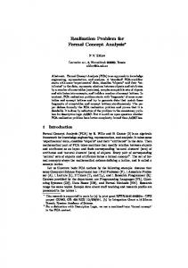
Figure 1: Computation time of exhaustively listing all minimal non-redundant association rules.

all three datasets we converted their nominal columns into binary attributes. For the sake of simplicity we are only interested in exact rules, i.e., rules with a confidence of 1. Figure 1 shows the required computation time for several minimum frequency thresholds using JClose [21] as a representative exhaustive method. Although there are more recent and potentially faster algorithms, all of them exhibit a similar behavior: the wellknown exponential increase of the required time with decreasing thresholds. Note that this explosion occurs already very early on the frequency scale. For Election the method becomes problematic for thresholds lower than 0.35. The situation for the other two datasets is even worse. For Questionnaire the required time for a threshold as high as 0.7 is more than five days! This demonstrates that even for moderately-sized datasets and moderate minimum support thresholds, finding association rules can be impossible. With a support threshold of 0.7 or higher, however, local pattern discovery becomes in fact global pattern discovery which is not desired in many applications [12]. There are even applications where one is interested exclusively in low support patterns (for instance see the study of Chow et al. on detecting privacy leaks using association rules [7]). Altogether, this motivates the development of algorithms that are capable of finding a designated small number of interesting patterns in feasible time. In particular, these patterns must not be restricted to high support patterns but should rather be selected according to application dependent quality measures. 1.3 Related Work and Challenges Exhaustive listing algorithms could be adapted to our task by (a) applying a post-processing step to select a subset of a given complete pattern collection that was previously

178

Copyright © by SIAM. Unauthorized reproduction of this article is prohibited.

listed (see [1, 26] for representative methods), by (b) aborting the pattern enumeration after the desired number of patterns have been generated, or by (c) directly restricting the search to high quality patterns (e.g., [20, 27]). As discussed in Section 1.2, approach (a) can be infeasible, approach (b) usually leads to a nonrepresentative set of patterns that depends on the internal search order of the listing scheme, and approach (c) usually suffers from computational complexity issues. For instance, finding k patterns of maximum frequency having a minimum length [24] or finding a pattern that is infrequent in one database but frequent in another [25] can neither exactly nor approximately be solved in polynomial time (unless P=NP). This is due to the hard thresholds respectively optimality requirements involved. Sampling algorithms can circumvent these negative complexity results by replacing hard thresholds with guaranteeing that the probability of a pattern to appear in the output is proportional to its quality. As a positive side-effect, the user is freed of the often troublesome task of finding appropriate thresholds. Al Hasan et al. [13] were the first to propose to circumvent the listing bottleneck by using randomized sampling. Their algorithm aims to generate a representative list of maximal frequent subgraphs of a given graph database by a twostep approach: first a number of maximal frequent subgraphs is randomly generated, and then a representative subset of this sample is selected based on a similarity measure. The sampling phase of this algorithm, however, provides no control over the target distribution. In contrast, the algorithm from [14] essentially simulates a Markov chain with uniform stationary distribution. While the process described there is also used to sample maximal frequent subgraphs, its actual state space is the set of all frequent subgraphs. A similar chain has been used in [5] for the purpose of quickly counting the number of frequent sets without listing them. There is no straightforward way of adapting these processes to sampling closed sets. Using a set sampler within a rejection sampling approach does not lead to an efficient algorithm because the number of sets can grow exponentially in the number of closed sets. Consequently, the probability of successfully drawing a closed set with rejection sampling can be very small; for a small database like “msweb” from the UCI machine learning repository [2] with 285 items and 32K transactions already as small as 10−80 . Similarly, mapping a drawn itemset to its smallest closed superset, is not a viable option: the varying number of generators among the closed set would introduce an uncontrollable bias. This motivates the construction of a random walk algorithm that directly uses the closed sets as state space.

2 Background This section recalls definitions from formal concept analysis (FCA) and closed set mining as well as Markov chains. FCA and closed set mining are strongly related. In this work we prefer the notions of FCA because of its symmetric treatment of items and transactions, which simplifies the subsequent technical discussion. For more information on FCA we refer to Wille’s textbook [9], for Markov chains to Randall’s survey [22] and references therein. 2.1 Formal concept analysis Let X be some set. We denote the power set of X by P(X). A mapping σ : P(X) → P(X) is called a closure operator if it satisfies for all A ⊆ B ⊆ X extensivity, i.e., A ⊆ σ(A), monotonicity, i.e., σ(A) ⊆ σ(B), and idempotence, i.e., σ(A) = σ(σ(A)). The set of all closed sets of σ, i.e., its fixpoints, is denoted by σ(P(X)). A (formal) context is a tuple (A, O, D) with A and O finite sets referred to as attributes and objects, respectively, and D ⊆ A × O a binary relation. In closed set mining, A, O, and D are referred to as items, transactions, and database, respectively. The maps O[·] : P(A) → P(O) and A[·] : P(O) → P(A) are O[X] = {o ∈ O : ∀a ∈ X, (a, o) ∈ D} and A[Y ] = {a ∈ A : ∀o ∈ Y, (a, o) ∈ D} , respectively. An ordered pair C = (I, E) ∈ P(A)×P(O) is called a (formal) concept, denoted hI, Ei, if O[I] = E and A[E] = I. The set I is called the intent of C and E is called its extent. The set of all concepts for a given context is denoted C(A, O, D) or just C when there is no ambiguity. It is partially ordered by the binary relation  defined by hI, Ei  hI 0 , E 0 i if and only if I ⊆ I 0 (or equivalently E ⊇ E 0 ). For the minimal respectively maximal elements of C with respect to  we write “⊥” for hA[O] , Oi and “>” for hA, O[A]i. It is well-known that

179

a) the maps A[·] and O[·] form an (order-reversing) Galois connection, i.e., X ⊆ A[Y ] ⇐⇒ Y ⊆ O[X] , b) their compositions φ = A[O[·]] and ψ = O[A[·]] form closure operators on P(A) and P(O), respectively, c) and all concepts C = hI, Ei ∈ C are of the form C = hφ(X), A[φ(X)]i for some X ⊆ A respectively C = hO[ψ(Y )] , ψ(Y )i for some Y ⊆ O, i.e., the intents of all concepts are the closed sets of φ and the extents the closed sets of ψ.

Copyright © by SIAM. Unauthorized reproduction of this article is prohibited.

2.2 Markov chains Monte Carlo Methods A (discrete) Markov chain on state space Ω is a sequence of discrete random variables (Xt )t∈N with domain Ω satisfying the Markov condition, i.e., that P[Xt+1 = x|X1 = x1 , . . . , Xt = xt ] is equal to P[Xt+1 = x|Xt = xt ] for all t ∈ N and x, x1 , . . . , xt ∈ Ω satisfying P[X1 = x1 , . . . , Xt = xt ] > 0. The uniform distribution on Ω is denoted u(Ω). In this article we only consider time-homogeneous Markov chains on finite state spaces. Given a probability distribution on the initial state, the joined distribution of (Xt )t∈N is completely specified by the state transition probabilities p(x, y) = P[Xt+1 = y|Xt = x] of all x, y ∈ Ω, which do not depend on t. Let pt (x, y) denote the t-step probability, i.e., pt (x, y) = P[Xn+t = y|Xn = x]. We call a state y ∈ Ω reachable from a state x ∈ Ω if there is a t ∈ N such that pt (x, y) > 0. The chain (Xt )t∈N is called aperiodic if for all x, y ∈ Ω with x is reachable from y there is a t0 ∈ N such that for all t ≥ t0 it holds that pt (x, y) > 0, and it is called irreducible if any two states are reachable from one another. Finally, (Xt )t∈N is called ergodic if it is irreducible and aperiodic. Any ergodic Markov chain has a unique limiting stationary distribution π : Ω → [0, 1], i.e., for all states x, y ∈ Ω it holds that limt→∞ pt (x, y) = π(y). Moreover, if there is a distribution π 0 : Ω → [0, 1] satisfying the detailed balance condition

unsupervised settings, e.g., association rule discovery, as well as scores used in supervised descriptive rule induction tasks such as emerging pattern mining [25], contrast set mining [4], or subgroup discovery [6]. For coherence we define all notions from the perspective of FCA. Let (A, O, D) be a context. We consider two types of local patterns: simple sets of attributes F ⊆ A, and association rules X → Y with X, Y ⊆ A. There are many measures in the literature for ranking patterns according to their interestingness. The support of a set F ⊆ A is the relative size of its extent, i.e., qsupp (F ) = |O[F ]| / |O|. A measure that is based on the minimum description length principle is the area function [11], i.e., qarea (F ) = |F | |O[F ]|. The support of a rule X → Y is defined as the support of X ∪ Y , and its confidence is qconf (X → Y ) = |O[X ∪ Y ]| / |O[X]|. We sometimes denote the c confidence of a rule above its →-symbol, i.e., X → Y . Rules with a confidence of 1 are called implications or exact rules. In order to define supervised evaluation measures one assumes that there are associated binary labels l(o) ∈ {+, −} for all objects o ∈ O. Patterns F ⊆ A can then be ranked according to the distributional unusualness of these labels on the pattern’s extent, respectively according to their support difference between the positive and the negative portion of the objects. A repre(2.1) ∀x, y ∈ Ω, π 0 (x)p(x, y) = π 0 (y)p(y, x) sentative measure is the binomial quality function   + and p is irreducible then π 0 is a stationary distribution |O [F ]| |O+ | − qbino (F ) = qsupp (F ) and p is called time-reversible. |O[F ]| |O| A Markov chain Monte Carlo method generates an element from Ω according to π by simulating (Xt )t∈N for where (A, O+ , D+ ) denotes the sub-context containing some time starting in an arbitrary state X0 = x0 ∈ Ω. only the objects with positive labels, i.e., O+ = {o ∈ O : Clearly, for that approach to be effective one has to (a) l(o) = +} and D+ = {(a, o) ∈ D : o ∈ O+ }. be able to efficiently generate a “neighbor” y ∼ p(x, ·) For both kinds of evaluation measures— for a given state x and (b) know after how many sim- unsupervised and supervised—it has been shown ulation steps t the distribution of Xt is “close enough” that by considering only closed sets, i.e., sets F ⊆ A to π. The distance from the t-step distribution of a with F = φ(F ), one can focus on non-redundant rule Markov chain with X0 = x to its stationary distribu- families. In particular for association rules, a rule c tion can be measured by the total variation distance X → Y is called minimal non-redundant if there is no P c kpt (x, ·), πktv = 1/2 y∈Ω |pt (x, y) − π(y)|. Using this rule X 0 → Y 0 with X 0 ⊆ X, Y 0 ⊇ Y and the same definition the mixing time of (Xt )t∈N is defined by support. The following result of [3] relates closed sets to exact minimal non-redundant association rules. τ () = max min{t0 ∈ N : ∀t ≥ t0 , kpt (x, ·), πktv ≤ } x∈Ω Proposition 1. (Bastide et al.) All exact minimal as the minimum number of steps one has to simulate non-redundant rules X → Y of a context (A, O, D) are (Xt )t∈N until the resulting distribution is guaranteed to of the form Y = φ(Y ) with X being a minimal set with φ(X) = Y . be -close to its stationary distribution. 2.3 Closed Local Pattern Mining Finally, we fix 3 Sampling Concepts notions and notations of closed local pattern mining and We are now ready to describe our concept sampling their evaluation metrics. This includes scores used in algorithm. First, we show how the state space, i.e.,

180

Copyright © by SIAM. Unauthorized reproduction of this article is prohibited.

D a b c d the concept lattice of a given context, can be connected 1 0 1 1 0 in a way that allows to efficiently select a random 2 1 0 1 0 element from the neighborhood of some concept. We 3 1 1 0 0 achieve this by using the closure operators induced by 4 1 1 0 1 the context. Then, in a second step, we apply to this 5 0 0 0 1 initial idea the Metropolis-Hastings algorithm and show that the resulting Metropolis process is irreducible. It can therefore be used to sample a concept according to Table 2: Example context with attributes {a, b, c, d} and any desired strictly positive distribution. objects {1, 2, 3, 4, 5}. 3.1 Generating Elements In order to construct a stochastic process on the concept lattice of a given context we will exploit its associated closure systems. More specifically, one can “move” from one closed set of a closure operator to another by a single element augmentation and a subsequent closure operation. In this context, we refer to the involved single elements as generating elements that can be defined as follows. Definition 1. (Generating Element) Let σ be a closure operator on P(X) and C, C 0 ∈ σ(P(X)) be closed sets. We say that an element x ∈ X generates C 0 from C with respect to σ if σ(C ∪ {x}) = C 0 . The set of all such generating elements is denoted by Gσ (C, C 0 ). These generating elements can be used to define a directed graph on the family of closed sets in which two vertices C, C 0 are joined by an arc if there is at least one element generating C 0 from C. This graph is implicitly traversed by several closed set listing algorithms. Definition 2. (Generator Graph) Let σ be a closure operator on P(X). The generator graph Gσ = (C, Eσ , lσ ) of σ is the directed labeled graph on the closed sets C = σ(P(X)) as vertices with edges Eσ = {(C, C 0 ) ∈ C × C : Gσ (C, C 0 ) 6= ∅} ,

generator graphs to a given context—the one induced by φ and the one induced by ψ. For the example context from Table 2 these graphs are drawn in Figure 2. Note that the arc relation Gφ is generally not identical to the transitive reduction of , which is usually used within diagrams illustrating a concept lattice: the concepts ha, 234i and habd, 4i are joined by an arc although they are not direct successors with respect to . The basic idea for our sampling algorithm is to perform a random walk on these generator graphs. Taking just one of them, however, does not result in an irreducible chain. Either > or ⊥ would be an absorbing state for such a process, in which any random walk will result with a probability converging to 1 for an increasing number of steps. A first idea to achieve irreducibility might be to take one of the corresponding generator graphs, say Gφ , add all inverse edges of Eφ as additional possible state transitions, and perform a random walk on the resulting strongly connected graph. Unfortunately, with this approach, drawing a neighbor of a given concept (as required for an efficient chain simulation) is as hard as the general problem of sampling a concept.

Proposition 2. Given a context (A, O, D) and a conand with edge labels lσ : E → P(X) equal to the cept hI, Ei ∈ C, drawing a predecessor of hI, Ei in Gφ generating elements, i.e., lσ (C, C 0 ) = Gσ (C, C 0 ). uniformly at random, i.e., a concept hI 0 , E 0 i ∈ C with φ(I 0 ∪ a) = I for some a ∈ A, is as hard as generating It is easy to see that Gφ is a) acyclic except for self-loops an arbitrary element of C uniformly at random. and b) rooted in σ(∅): statement a) follows by observing 0 0 that (C, C ) ∈ Eσ implies C ⊆ C , and for b) note Proof. A given context (A, O, D) with concepts C can be that for all closed sets C = {x1 , . . . , xk } the sequence transformed into a context (A0 , O0 , D0 ) with concepts C 0 x1 , . . . , xk corresponds to an edge progression (walk) as follows: set A0 = A∪{a∗ } with a∗ 6∈ A, O0 = O∪{o∗ } from σ(∅) to C due to extensivity and monotonicity with o∗ 6∈ O, and of σ. A random walk on the generator graph can be performed by the following procedure: in a current D0 = D ∪ {(a, o∗ ) : a ∈ A0 } . closed set Y ∈ σ(P(X)) draw an element x ∼ u(X), and then move to σ(Y ∪{x}). The transition probability Then C = C 0 \{hA0 , {o∗ }i} and for all hI, Ei ∈ C, it holds from a set Y to a set Z is then directly proportional to that φ0 (I ∪ {a∗ }) = A0 , i.e., all C ∈ C are predecessors the number of generating elements |Gσ (Y, Z)| and can of hA0 , {o∗ }i in Gφ0 .  be computed efficiently. Now, if one identifies concepts with their intents An alternative approach is to use the a random walk respectively with their extents, there are two associated on the union of both generator graphs as stochastic

181

Copyright © by SIAM. Unauthorized reproduction of this article is prohibited.

A {}

A {} 3 4

c

c

a,d

abd 4 d

c

2

abd 4

2

d d

1

bc 1

ac 2

d

ab 34

a,b

bc 1

ac 2

3,4

3,4

1

1 b a

a 234

a

b 134

2

2

b

c

c

5

3

b,d

ab 34

1 5

a 234

d 45

c 12

5

b 134

c 12

d 45

5

2,5 a

c

b

3,4,5

d

1,5

{} O

5

(a)

{} O

1,2,3

(b)

Figure 2: Generator graphs Gφ and Gψ (drawn without self-loops) for the context from Table 2.

in Figure 2 shows that the union of the two generator graphs corresponding to a given context does not necessarily induce symmetric state transition probabilities. In fact, the resulting process is in general not even time-reversible—see for instance concepts ⊥ and hbc, 1i in Figure 2, for which we have q(⊥, hbc, 1i) = 0 but q(hbc, 1i , ⊥) > 0. As a solution one can factor the quotient of the proposal probabilities into the acceptance probabilities. The resulting state transitions are ( π(C 0 ) 0 0 for concepts C = hI, Ei and C 0 = hI 0 , E 0 i. It is easy p(C, C 0 ) = q(C, C ) min{α π(C) , 1}, if q(C, C ) > 0 to see that the resulting stochastic process is an ergodic 0, otherwise Markov chain. Thus, it has a stationary distribution to which it converges. Generally, however, we do not know where α = q(C 0 , C)/q(C, C 0 ). This is the Metropolisanything about this distribution. In the next subsection Hastings algorithm [15], and the underlying process is we show how the chain can be modified such that it called the Metropolis-process of q and π. For the exconverges to a distribution that is known and desired. ample from Table 2 its state transition probabilities are drawn in Figure 3. It is important to note that, in or3.2 Metropolis-Hastings Algorithm Let π : C → der to simulate the Metropolis process, one does not [0, 1] be the desired target distribution, according to need the exact probabilities π(C 0 ) and π(C). As the which we would like to sample concepts. For techni- acceptance probability only depends on their quotient, cal reasons that will become clear shortly we require π it is sufficient to have access to an unnormalized potento be strictly positive, i.e., π(C) > 0 for all C ∈ C. In tial f : C → R such that there is a constant α with practice this can be achieved easily. If our ergodic pre- f (C) = απ(C) for all C ∈ C. For instance, for the uniliminary chain would have symmetric state transition form target distribution one can choose any constant probabilities, we could simply use it as proposal chain function f . Algorithm 1 is a Markov chain Monte Carlo as follows: in a current concept C, propose a successor implementation of the Metropolis process. It takes as C 0 according to q, and then accept the proposal with input a context, a number of iterations s, and an oracle probability π(C 0 )/π(C). This is the classic Metropolis for the unnormalized potential f . Then, after choosing algorithm, and for the resulting Markov chain it is easy an initial state X0 uniformly among ⊥ and >, it simto check that it satisfies the detailed balance condition ulates the process for s steps, and returns the state it for π—granted that q is symmetric as well as ergodic has reached by that time, i.e., its realization of Xs . and that π is strictly positive. However, the example It is easy to see that the algorithm indeed uses the process. Technically, this can be realized as follows: in a current state flip a fair coin and then, based on the outcome, choose either Gφ or Gψ to proceed to the next state as described above. This leads to the state transition probabilities  0  if C ≺ C 0 |Gφ (I, I )| /(2 |A|), 0 0 q(C, C ) = |Gψ (E, E )| /(2 |O|), if C  C 0   |I| /(2 |A|) + |E| /(2 |O|), if C = C 0 .

182

Copyright © by SIAM. Unauthorized reproduction of this article is prohibited.

Theorem 3. On input context (A, O, D), step number s, and strictly positive function f , Algorithm 1 produces in time O(s |D|) a concept C ∈ C(A, O, D) according to a distribution psf such that

0.1 0.07 1/10

1/10

1/10

0.1

1/10

1/10

0.09 1/10

lim kpsf , πktv = 0

1/10

s→∞ 0.1

1/10

0.07

0.1

0.1 0.08

1/10

0.08

1/8

1/10

1/10

1/8 0.1

1/8

1/10

0.1 0.11

0.11

1/8

where π is the distributionPon C resulting from normalizing f , i.e., π(·) = f (·)/ C∈C f (C).

1/10

0.1

0.1

0.13

0.13

1/8

1/8

1/8 0.1 0.15

Figure 3: Resulting state transitions for Table 2 and f (·) ≡ 1; remaining probabilities are assigned to selfloops; nodes contain stationary probability (black) and apx. probability after five steps with X0 = h∅, Oi (grey).

Proof. The time complexity is easy to see. Also, by construction, it can directly be checked that π and p satisfy the detailed balance condition (Eq. 2.1). It remains to show irreducibility, i.e., pt (hI, Ei , hI 0 , E 0 i) > 0 for some t and all pairs of concepts hI, Ei , hI 0 , E 0 i ∈ C. It is sufficient to consider the case hI, Ei  hI 0 , E 0 i: for other states reachability follows then via hI ∩ I 0 , A[I ∩ I 0 ]i  hI, Ei, hI ∩ I 0 , A[I ∩ I 0 ]i  hI 0 , E 0 i, and the transitivity of reachability. Moreover, as the considered state spaces C are finite, it suffices to consider direct suc. 0 cessors hI, Ei  hI , E 0 i. For such concepts it is easy to show that I is a maximal proper subset of I 0 in φ(P(A)) and E 0 is a maximal proper subset of E in ψ(P(O)). Let a ∈ I 0 \ I and o ∈ E \ E 0 . It follows by the closure operator properties that φ(I ∪ {a}) = I 0 and ψ(E 0 ∪ {o}) = E. Thus, the proposal probabilities between hI, Ei and hI 0 , E 0 i are non-zero in both directions, and together with the fact that f is strictly positive, it follows for the transition probability of the Metropolisprocess that p(hI, Ei , hI 0 , E 0 i) > 0 as required. 

state transition probabilities p. So far, however, we omitted an important aspect of its correctness: while π satisfies the detailed balance condition for this chain, this comes at the cost of setting p(C, C 0 ) = 0 for some pairs of concepts that have q(C, C 0 ) > 0. Thus, the irreducibility of q is not directly implied by the irreducibility of p. It is, however, guaranteed by the closure properties of φ and ψ, as shown in the proof of the following summarizing theorem. Now that we know that our algorithm asymptotically draws samples as desired, it remains to discuss, for how Algorithm 1 Metropolis-Hastings Concept Sampling many steps one has to simulate the process until the distribution is “close enough” to the target distribution. Input : context (A, O, D), number of iterations s, oracle of map f : C → R+ 3.3 Number of Iterations Unfortunately, in the Output : concept hI, Ei worst case the mixing can be infeasible slow, i.e., require 1. init hI, Ei ∼ u({>, ⊥}) and i ← 0 a number of steps that can grow exponentially in the 2. i ← i + 1 input size. The following statement on the mixing time 3. draw d ∼ u({up, down}) holds. 4. if d = up then Proposition 4. Let  > 0 be fixed and τn () denote the 5. draw a ∼ u(A) worst-case mixing time of Algorithm 1 for the uniform 6. hI 0 , E 0 i ← hφ(I ∪ {a}), O[φ(I ∪ {a})]i target distribution and an input context of size n. Then 7. α ← (|Gψ (E 0 , E)| |A|) / (|Gφ (I, I 0 )| |O|) τn () ∈ Ω(2n/2 ). 8. else 9. draw o ∼ u(O) Proof. We prove the claim by showing that for all n with 10. hI 0 , E 0 i ← hA[ψ(E ∪ {o})] , ψ(E ∪ {o})i an even integral square root √ there is a context (A, O, D) 11. α ← (|Gφ (I 0 , I)| |O|) / (|Gψ (E, E 0 )| |A|) with A = O = {1, . . . , n} and |D| = n/2 − n such 12. draw x ∼ u([0, 1]) that τ () ≥ 2n/2−3 log(1/(2)). It is well-known (see for 13. if x < αf (I 0 ) / f (I) then hI, Ei ← hI 0 , E 0 i instance [22]) that the mixing time of a Markov chain 14. if i = s then return hI, Ei else goto 2 with state space C and stationary distribution π is lower bounded by (3.2)

183

τ () ≥ 1/(4Φ) log(1/) ,

Copyright © by SIAM. Unauthorized reproduction of this article is prohibited.

where Φ is the conductance defined as the minimum number ΦS over all P S ⊆ C with π(S) ≤ 1/2 where ΦS is equal to (1/π(S)) x∈S,y∈C\S π(x)p(x, y). Choose D = {(i, j) : i 6= j, (i, j ≤

√ √ n/2 ∨ i, j > n/2)} .

Then the set of concepts is a disjoint union C(A, O, D) = . C1 ∪ C2 with √ C1 ={hI, O[I]i : I ⊆ {1, . . . , n/2}} √ √ C2 ={hI, O[I]i : ∅ 6= I ⊆ { n/2 + 1, . . . , n}} ∪ {>} and if π is the uniform distribution, it holds that π(C1 ) = 1/2. Moreover,√ the only state pairs that contribute to ΦC1 are the n pairs {⊥, C} and {C 0 , >} of the form √ √ C ∈ {hI, Ei : I ∈ {{ n/2 + 1}, . . . , { n}}} √ C 0 ∈ {hA \ {a}, Ei : a ∈ {1, . . . , n/2}} . Consequently, 1/2n/2−1 = ΦC1 ≤ Φ and with (3.2), τ () ≥ 2n/2−3 log(1/(2)) as required. 

Figure 4: Distribution convergence.

Thus, even the strictest theoretical worst-case bound on the mixing time for general input contexts would not lead to an efficient algorithm. The proof of the proposition is based on the observation that the chain can have a very small conductance, i.e., a relatively large portion of the state space (growing exponentially in n) can only be connected via a linear number of states to the rest of the state space. We assume that real-world datasets do not exhibit this behavior. In our applications we therefore use the following heuristic polynomially bounded function for assigning the number of simulation steps:

This can also be observed in our experiments with four real-world databases 1 and two target distributions: the uniform distribution and the distribution proportional to the area quality measure π(·) = qarea (·)/Z. The results are illustrated in Figure 4. Note that the plots differ in their semantics. While for both target distributions a point (x, y) means that the x-step distribution has a total variation distance of y from the target distribution, for the heuristic the inverse of the step-heuristic is shown, i.e., the value of  on the y-axis reflects the desired accuracy that leads to a particular number of steps. Thus, the heuristic was “correct” if its corresponding plot dominates the two total variation distance plots. As we can see, this was the case for both distributions on all four datasets. In fact, the heuristic was rather conservative. Note that the y-axis has a logarithmic scale. The effect of the target distribution on the mixing time is unclear. On the one hand, deviation from the uniform distribution can create bottlenecks, i.e., low conductance sets, where there have been non before. On the other hand, it can also happen that bottlenecks of the uniform distribution are softened. This can be observed for “mushroom” and “chess”. For that reason we do not reflect the target distribution in our heuristic.

steps((A, O, D), ) = 4n ln(n) ln() where n = min{|A| , |O|}. The motivation for this is as follows (see also [5], where a similar heuristic is used). Assume without loss of generality that |A| < |O|. As long as only “d = up” is chosen in line 3 of the algorithm the expected number of steps until all elements of A have been drawn at least once is n ln(n) + O(n) with a variance that is bounded by 2n2 (coupon collector’s problem). It follows that asymptotically after 2n ln(n) all elements have been drawn with probability at least 3/4. Consequently, as “d = up” is chosen with probability 1/2, we can multiply with an additional factor of 2 to know that with high probability there was at least one step upward and one step downward for each attribute a ∈ A—if one assumes a large conductance this suffices to reach every state with appropriate probability. The final factor of ln() is motivated by the fact that the total variation distance usually decays exponentially in the number of simulation steps.

1 Databases are from UCI Machine Learning Repository [2]. In order to explicitly compute the state transition matrices we had to use only a sample of the transactions for three of the databases. The sample size is given in brackets.

184

Copyright © by SIAM. Unauthorized reproduction of this article is prohibited.

4 Concept Counting In this section we highlight the connection of concept sampling to concept counting. This connection is important because it ties the complexities of these two tasks together. In particular, we show how concept sampling can be used to design a randomized approximation scheme for the number of concepts of a given context, i.e., a randomized algorithm that produces for an input context (A, O, D) and  ∈ (0, 1/2] a number N such that (1 − ) |(A, O, D)| ≤ N ≤ (1 + ) |(A, O, D)| with probability at least 3/4. Beside theoretical insight, the motivation for this is that such an algorithm can be used to quickly check the feasibility of an potentially exponential time exhaustive listing of all concepts (see also [5] where the same problem is discussed for frequent itemsets). Let (A, O, D) be a context and o1 . . . , om some ordering of the elements of O. For i ∈ {0, . . . , m} define the context Ci = (A, Oi , Di ) with Oi = {oj : j ≤ i}, Di as the restriction of D to Oi , φi as the corresponding attribute closure operator, and Ii = φi (P(A)) the concept intents. Note that in general a concept intent I ∈ Ii+1 is not an intent of a concept with respect to the context Ci , i.e., not a fixpoint of φi . The following two properties, however, hold.

complete context as (4.3)

|C(A, O, D)| =

|Io |

m Y

!−1 |Ii−1 | / |Ii |

.

i=1

For i ∈ {1, . . . , m} let Zi (I) denote the binary random variable on measure space (Ii , πi ) that takes on value 1 if I ∈ Ii−1 and 0 otherwise. Independent simulations of these random variables can be used to count the number of concepts Qm via Equation 4.3 using the product estimator Z = 1 Z¯i where (1) (t) Z¯i = (Zi + · · · + Zi )/t (j)

with Zi independent copies of Zi . Using standard reasoning (see, e.g., [17]) and Lemma 5 one can show that Z is -close to |C(A, O, D)| with probability at least 3/4 if (i) the total variation distance of the πi to the uniform distribution on Ii is not greater than /(12 |O|) and (ii) t ≥ 12 |O| /2 . See Algorithm 2 for a pseudocode simulating this estimator. Observing that the roles of A and O are interchangeable, i.e., the number of concepts of (A, O, D) is equal to the number of concepts of the “transposed” context, we can conclude:

Theorem 6. There is a randomized approximation scheme for the number of concepts |C| of a given context
(A, O, D) with time complexity O n−2 TS (/(12n)) for accuracy  where n = min(|A| , |O|) and TS (0 ) is the time required to sample a concept almost uniformly, i.e., Lemma 5. For all contexts (A, O, D) and all i ∈ according to a distribution with a total variation dis{0, . . . , |O|} it holds that (i) Ii ⊆ Ii+1 and (ii) 1/2 ≤ tance of at most 0 from uniform. |Ii | / |Ii+1 |.

Proof. For (i) let I ∈ Ii . In case oi+1 6∈ I[Oi+1 ], it is I[Oi+1 ] = I[Oi ]. Otherwise, per definition we know that all a ∈ A that satisfy (a, o) ∈ D for all o ∈ Oi are also satisfying (a, o) ∈ D for all o ∈ Oi+1 . Thus, in both cases φi+1 (I) = A[Oi+1 [I]] = A[Oi [I]] = φi (I) = I as required. We prove (ii) by showing that the restriction of the closure operator φi to Ii+1 \ Ii is an injective map into Ii , i.e., |Ii+1 \ Ii | ≤ |Ii |. Together with (i) this implies the claim. Assume for a contradiction that there are distinct intents X, Y ∈ Ii+1 \ Ii such that φi (X) = φi (Y ). Then Oi [X] = Oi [Y ], and, as X and Y are both closed with respect to φi+1 but not closed with respect to φi , it must hold that oi+1 ∈ Oi+1 [X] ∩ Oi+1 [Y ]. It follows that Oi+1 [X] = Oi [X] ∪ {oi+1 } as well as Oi+1 [Y ] = Oi [Y ] ∪ {oi+1 }. This implies Oi+1 [X] = Oi+1 [Y ] and in turn X = Y contradicting the assumption that the intents are distinct. 

Algorithm 2 Concept Counting Input : context (A, O, D), accuracy  ∈ (0, 12 ] steps(Ci ,0 ) Require: kpi,1 , u(Ci )ktv ≤ 0 for all i and 0 Output : q with P[(1−) |C| ≤ q ≤ (1+) |C|] ≥ 3/4 1. 2. 3. 4. 5. 6. 7. 8.

t ← 12 |O| /2 for i = 1, . . . , |O| do ri ← 0 for k = 1, . . . , t do hI, Ei ← sample(Ci , steps(Ci , /(12 |O|)), 1) if φi−1 (I) = I then ri ← ri + 1 ri ← ri /t Q|O| −1 return i=1 ri

To evaluate the accuracy of this randomized counting approach, we executed a series of runs on the chess dataset and compared the estimate computed by our randomized algorithm with the exact number of conThus, the Ii define an increasing sequence of closed set cepts. We did not consider the whole dataset but infamilies with |I0 | = |{A}| = 1 and |Im | = |C(A, O, D)| stead used samples of different size. We used an accuthat allows to express the number of concepts of the racy of  = 0.5. The result is shown in Figure 4. On the

185

Copyright © by SIAM. Unauthorized reproduction of this article is prohibited.

sampling wrt. qsupp sampling wrt. qarea JClose... ... with support

Election 2.1 sec. 2.2 sec. 59 min. 0.35

Questio. 21 min. 21 min. 7500 m. 0.7

Census 7 min. 7 min. 1729 min. 0.7

Table 3: Time for association rule generation.

Figure 5: Estimated number of concepts on samples of the ’chess’ dataset.

x-axis, we give the size of the sample, while the y-axis shows the exact number of concepts (“exact count”), the upper and lower 0.5 deviation limits (“upper limit” and “lower limit”), as well as the result of the randomized algorithm in a series of 10 runs per sample (“estimated count”). The figure shows that in all randomized runs, the approximated result lies within the given deviation bound. This is a further positive evaluation of the step heuristic developed in Section 3.3. 5 Application to Local Pattern Mining In this section, we will present exemplary applications of the sampling algorithm to local pattern mining. This revisits the motivations from Section 1.2. 5.1 Association Rule Mining First, we illustrate how the sampling algorithm can be used in the context of minimal non-redundant association rule discovery (see Section 2). Again, for the sake of simplicity, we consider exact association rules, i.e., rules with a confidence of 1. Sampling a rule with confidence below 1 can be done, for instance, by sampling the consequence of the rule in a first step; and then sampling the antecedent according to a distribution that is proportional to the confidence and support of the resulting rule. Based on Proposition 1, we can generate exact minimal non-redundant association rules by first sampling a concept hY, Ei, and then calculating a minimal generator X of the concept’s intent, i.e., a minimal set with φ(X) = Y . For the calculation of the minimal generators, we use a simple greedy algorithm that is essentially equivalent to the greedy algorithm for the set cover problem (see [6] for a discussion). In fact, with this algorithm we generate an approximation to a shortest generator and not only a minimal generator with respect to set inclusion. Thus, we are aiming for particularly short rule antecedents.

With this method we generate association rules for the three datasets Election, Questionnaire, and Census from Section 1.2 (see Table 1) for two different target distributions: the one proportional to the rule’s support and the one proportional to their area (adding the constant 1 to ensure a strictly positive distribution). That is, we used f = qsupp respectively f = qarea (see Section 2) as parameter for Algorithm 1. As desired closeness to the target distribution we choose  = 0.01. Note that, in contrast to exhaustive listing algorithms, for the sampling method we do not need to define any threshold like minimum support. Table 3 shows the time required to generate a single rule according to qsupp and qarea . In addition, the table shows the runtime of JClose for exemplary support thresholds. Comparing the runtimes for sampling with that of JClose, we can see that the uniform generation of a rule from the Election dataset takes about 1/1609 of the time needed to exhaustively list non-redundant association rules with threshold 0.35. For Questionnaire and threshold 0.7, the ratio is 1/340; finally for Census with threshold 0.7, the ratio is 1/247. As discussed in Section 1.2, all exhaustive listing algorithms exhibit a similar asymptotic performance behavior. Thus, for methods that outperform JClose on these particular datasets, we would end up with similar ratios for slightly smaller support thresholds. Moreover, it is not uncommon that one is interested in a small set of rules having a substantially lower support than the thresholds considered above. For such cases the ratios would increase dramatically, because the time for exhaustive listing increases exponentially whereas the time for sampling remains constant. Thus, for such applications sampling has the potential to provide a significant speedup. In fact, it is applicable in scenarios where exhaustive listing is hopeless. 5.2 Supervised Descriptive Rule Induction As second application we consider supervised descriptive rule induction, i.e., local pattern mining considering labeled data such as emerging pattern mining, contrast set mining, or subgroup discovery (see Section 2). This can be done by choosing the binomial quality qbino as parameter for Algorithm 1. In fact, we cap

186

Copyright © by SIAM. Unauthorized reproduction of this article is prohibited.

dataset sick soyb. lung.

#rows 3772 683 32

#cols. 27 35 56

#attr. 66 133 159

size 299K 199K 10K

target sick br.-spot ‘1’

best quality sampled quality

sick 0.177 0.167

soybean 0.223 0.187

lung. 0.336 0.263

Table 6: Best quality among all patterns versus best quality among sampled patterns.

Table 4: Databases for the supervised descriptive rule induction experiments.

sampling time listing time

sick 3 1460

soyb. 1 705

lung. 0.02 69

Table 5: Time (in seconds) of random pattern generation according to qbino compared to exhaustive listing. qbino from below by a small constant c to ensure a strictly positive target distribution, i.e., we use f (·) = max{qbino (·), c}. With the binomial quality function we have an evaluation metric that has shown to adequately measure interestingness in several applications. Thus, in addition to the computation time, in this experiment we can also evaluate the quality of the sampled patterns. We consider three labeled datasets from the UCI machine learning repository (listed in Table 4). As baseline method we use exhaustive closed subgroup discovery based on generator graph traversal [6]. This algorithm explores the same state space as the sampling algorithm and outperforms other (non-closed) listing algorithms on the considered datasets. Table 5 gives the time needed to generate a pattern by the randomized algorithm compared to the time for exhaustively listing all patterns with a binomial quality of at least 0.1. This threshold is approximately one third of the binomial quality of the best patterns in all three datasets. As observed in the unsupervised setting, the randomized approach allows to generate a pattern in a fraction of the time needed for the exhaustive computation. In order to evaluate the pattern quality, we compared the best patterns within a set of 100 samples to the globally best patterns (Table 6). Although the quality of the randomly generated patterns do not reach the optimum, we observe the anticipated and desired result: the collected subgroups form a high quality sample relatively to the complete pattern space, from which they are drawn. 6 Discussion We presented a Metropolis-Hastings algorithm able to effectively generate concepts according to some desired target distribution. In several exemplary applications we demonstrated how this algorithm can be used for

knowledge discovery and approximate counting. It is important to note that although we restricted the presentation to closed sets, the approach is not limited to this scenario. In fact it can be applied to all pattern classes having a similar Galois connection between patterns and transactions. Furthermore, the method can be combined with any anti-monotone or monotone constraint. It is for instance easy to see that the algorithm is still correct when the chain is restricted to the set of all frequent concepts. Although the heuristic polynomial step number leads to sufficient results in our experiments, clearly one would prefer a polynomial sampling algorithm with provable worst-case guarantee. There is, however, some evidence that no such algorithm exists or that at least designing one is a difficult problem: as we have shown in Section 4, an algorithm that can sample concepts uniformly in polynomial time can be used to design a fully polynomial randomized approximation scheme (FPRAS) for counting the number of concepts for a given context. This problem is equivalent to counting the number of maximal bipartite cliques of a given bipartite graph, which is as hard as a complexity class called #RHΠ1 ⊂ #P (hardness result and complexity class both were introduced in [8]). Despite much interest for such algorithms in several research communities, there is no known FPRAS for any #RHΠ1 -hard problem. In the absence of feasible a priori bounds on the mixing time, there are several techniques that can be used not only to detect mixing but even to draw perfect samples, i.e., generated exactly according to the stationary distribution (see [16] and references therein). The most popular variant of these perfect sampling techniques is coupling from the past (CFTP). It can be applied efficiently if the chain is monotone in the following sense: the state space is partially ordered, contains a global maximal as well as a global minimal element, and if two simulations of the chain that use the same source of random bits are in state x and y with x ≤ y then also the successor state of x must be smaller than the successor state of y. Indeed, at first glance it appears that CFTP may be applied to our chain because its state space is partially ordered by  and always contains a global minimal element ⊥

187

Copyright © by SIAM. Unauthorized reproduction of this article is prohibited.

as well as a global maximal element >. Even for the uniform target distribution, however, the chain is not monotone. This can be observed in the example of Figure 2: denote by succd,5,0 (hI, Ei) the successor of hI, Ei when the random bits used by the computation induce the decisions d = down, o = 5, and p = 0. Then hbc, 1i  hA, ∅i whereas succd,5,0 (hbc, 1i) = hbc, 1i 6 hd, 45i = succd,5,0 (hA, ∅i). It is an open problem, how to define a Markov chain on the concept lattice that has monotone transition probabilities. Acknowledgements Part of this work was supported by the German Science Foundation (DFG) under the reference number ‘GA 1615/1-1’. References [1] Foto N. Afrati, Aristides Gionis, and Heikki Mannila. Approximating a collection of frequent sets. In KDD, pages 12–19. ACM, 2004. [2] A. Asuncion and D.J. Newman. UCI machine learning repository, 2007. [3] Yves Bastide, Nicolas Pasquier, Rafik Taouil, Gerd Stumme, and Lotfi Lakhal. Mining minimal nonredundant association rules using frequent closed itemsets. In Computational Logic - CL 2000, pages 972– 986. Springer, 2000. [4] Stephen D. Bay and Michael J. Pazzani. Detecting group differences: Mining contrast sets. Data Min. Knowl. Discov., 5(3):213–246, 2001. [5] Mario Boley and Henrik Grosskreutz. A randomized approach for approximating the number of frequent sets. In ICDM, pages 43–52. IEEE Computer Society, 2008. [6] Mario Boley and Henrik Grosskreutz. Non-redundant subgroup discovery using a closure system. In ECML/PKDD (2), pages 179–194. Springer, 2009. [7] Richard Chow, Philippe Golle, and Jessica Staddon. Detecting privacy leaks using corpus-based association rules. In KDD 2008, pages 893–901. ACM, 2008. [8] Martin Dyer, Leslie Ann Goldberg, Catherine Greenhill, and Mark Jerrum. The relative complexity of approximate counting problems. Algorithmica, 38(3):471–500, 2004. [9] Bernhard Ganter and Rudolf Wille. Formal Concept Analysis: Mathematical Foundations. Springer Verlag, 1999. [10] Gemma C. Garriga, Petra Kralj, and Nada Lavraˇc. Closed sets for labeled data. J. Mach. Learn. Res., 9:559–580, 2008. [11] Floris Geerts, Bart Goethals, and Taneli Mielik¨ ainen. Tiling databases. In DS, pages 278–289, 2004. [12] David Hand. Pattern detection and discovery. In Pattern Detection and Discovery, volume 2447 of LNAI, pages 1–12. Springer, 2002.

188

[13] Mohammad Al Hasan, Vineet Chaoji, Saeed Salem, J´er´emy Besson, and Mohammed Javeed Zaki. Origami: Mining representative orthogonal graph patterns. In ICDM, pages 153–162. IEEE Computer Society, 2007. [14] Mohammad Al Hasan and Mohammed Javeed Zaki. Musk: Uniform sampling of k maximal patterns. In SDM, pages 650–661. SIAM, 2009. [15] W. K. Hastings. Monte carlo sampling methods using markov chains and their applications. Biometrika, 57(1):97–109, 1970. [16] Mark Huber. Perfect simulation with exponential tails on the running time. Random Struct. Alg., 33(1):29– 43, 2008. [17] Mark Jerrum and Alistair Sinclair. The Markov chain Monte Carlo method: an approach to approximate counting and integration, pages 482–520. PWS Publishing Co., Boston, MA, USA, 1997. [18] A . Knobbe, B. Cr´emilleux, J. F¨ urnkranz, and M. Scholz. From local patterns to global models: the lego approach to data mining. In Proc. of the ECML PKDD 2008 LEGO Workshop, 2008. [19] Matthew V. Mahoney and Philip K. Chan. Learning rules for anomaly detection of hostile network traffic. In ICDM, page 601, Washington, DC, USA, 2003. IEEE Computer Society. [20] Shinichi Morishita and Jun Sese. Traversing itemset lattice with statistical metric pruning. In PODS, pages 226–236. ACM, 2000. [21] Nicolas Pasquier, Rafik Taouil, Yves Bastide, Gerd Stumme, and Lotfi Lakhal. Generating a condensed representation for association rules. Journal of Intelligent Information Systems, 24(1):29–60, January 2005. [22] Dana Randall. Rapidly mixing markov chains with applications in computer science and physics. Computing in Science and Engineering, 8(2):30–41, 2006. [23] Leander Schietgat, Fabrizio Costa, Jan Ramon, and Luc De Raedt. Maximum common subgraph mining: A fast and effective approach towards feature generation. In MLG, 2009. [24] J. Wang, J. Han, Y. Lu, and P. Tzvetkov. Tfp: an efficient algorithm for mining top-k frequent closed itemsets. Knowledge and Data Engineering, IEEE Transactions on, 17(5):652–663, May 2005. [25] Lusheng Wang, Hao Zhao, Guozhu Dong, and Jianping Li. On the complexity of finding emerging patterns. Theoretical Computer Science, 335(1):15–27, 2005. [26] Dong Xin, Jiawei Han, Xifeng Yan, and Hong Cheng. Mining compressed frequent-pattern sets. In VLDB, pages 709–720. VLDB Endowment, 2005. [27] Xifeng Yan, Hong Cheng, Jiawei Han, and Philip S. Yu. Mining significant graph patterns by leap search. In SIGMOD, pages 433–444. ACM, 2008.

Copyright © by SIAM. Unauthorized reproduction of this article is prohibited.