Many protocols for wireless sensor networks employ some form of the very ... National ICT Australia is funded through the Australian Government's Backing ... Gossiping is a simple protocol that uses probabilistic broadcast to send or request.
To appear in: 5th International Conference on AD-HOC Networks & Wireless
Formal Verification and Simulation for Performance Analysis for Probabilistic Broadcast Protocols Ansgar Fehnker and Peng Gao National ICT Australia? and University of New South Wales
Abstract. This paper describes formal probabilistic models of flooding and gossiping protocols, and explores the influence of different modelling choices and assumptions on the results of performance analysis. We use Prism, a model checker for probabilistic systems, for the formal analysis of protocols and small network topologies, and use in addition MonteCarlo simulation, implemented in Matlab, to establish if the results and effects found during formal analysis extend to larger networks. This combination of approaches has several advantages. The formal model has well defined synchronization primitives with clear semantics for modelling synchronous and asynchronous communication between nodes. Model checking of the probabilistic model determines exact probabilities and performance bounds, results that cannot be obtained by simulation, and even if the model is non-deterministic. The Monte-Carlo simulation can then be used to study effects that only emerge in larger networks, such as phase transition.
1
Introduction
Wireless sensor networks is an emerging field that has received a lot of attention in recent years. Characteristic features of wireless networks are that each they gather information about the network and the environment in a distributed fashion, and that nodes use multi-hop communication on an unreliable medium. Each node has its own processor, radio, antenna, and clock. The processors operate under tight energy restrictions because nodes are either battery operated or rely on abient energy sources. This combination of characteristics calls for simple and robust distributed algorithms, that require few computing cycles, and thus little processing power. Many protocols for wireless sensor networks employ some form of the very simple flooding protocol to acquire or distribute information. Flooding a message means that each node that receives a message, propagates it to all its neighbors by broadcast. This introduces an unnecessary redundancy, because a node may ?
National ICT Australia is funded through the Australian Government’s Backing Australia’s Ability initiative, in part through the Australian Research Council.
receive a message multiple times. Gossiping protocols introduce a random element to reduce this redundancy. Gossiping means that each node decides with a certain probability to forward a message on or not. This reduces the probability that a node receives a message multiple times, thus the redundancy and cost. The main tool in model based development to evaluate the performance of a protocol is simulation. Common simulators in the wireless domain are ns-2, Opnet, and Glomosim, but it is not uncommon to build a customized simulator, for example, in Java or Matlab. Flooding and gossiping protocols have been studied before, for example in [1–4]. It has been observed in [5] that different simulator can produce vastly different results, even for a simple protocol such as flooding. The reason is that simulators employ different models for the MAC and physical layers. The results of the simulators say as much about the protocol, as about the particular the lower level implementation of the simulator. Protocols are a traditional subject for analysis in formal methods, and wireless protocols are no exception. The model checker Prism, for example, has been used to analyse the randomized backoff procedure in the 802.11 wireless protocol [6]. Flooding and gossiping protocols were examined in [3] and [4]. The latter combine simulation studies and manual analytic evaluation. The formal analysis in [3] deals with the correctness of the protocol, while simulation is used to assess the performance. The analysis in [4] is manual for a general model of possible topologies, however, for a specific set of assumption on the synchronization. This paper uses model checking for performance analysis of flooding and gossiping protocols. Model checking has been used before for performance analysis, for example, [7] describes for example how Prism can be used to evaluate a strategy for dynamic power management, and [8] describes a tool based on model checking timed automata that evaluates schedulers for embedded systems. The main motivation of this paper is the observation that different papers on wireless protocols such as gossiping use different assumptions, which makes comparison of results difficult. For example, [3] and [5] both evaluate the flooding protocol, but sending and receiving is perfectly synchronized in [3], while [5] assumes a random waiting period in-between sending and receiving. In this paper we examine what effect this and similar choices have on the outcome of the analysis. This paper explores in particular the effect of collisions, unreliable channels versus probabilistic broadcast, and the influence of timing. This analysis can explain why the performance result of gossiping for a perfectly synchronized network without collision, are similar to the result on a network with randomized delay and collision, although the actual behavior is vastly different. The next section of this paper gives an introduction to flooding and gossiping protocols. Section 3 and 4 introduce the model checker Prism and Monte-Carlo simulation respectively. The models and the results will be presented in Section 5, and followed by a discussion and summary in Section 6. 2
2
Flooding and Gossiping
Gossiping is a simple protocol that uses probabilistic broadcast to send or request information in a wireless network. The gossiping protocol can be informally summarized as follows: – The source node broadcasts the message or request to all its neighbors. It then proceeds to sleep. – Nodes that receive a message chooses with probability psend to forward the received message, and with probability 1 − psend to ignore the message. In either case the node proceeds to sleep. Gossiping is equal to flooding, if psend is equal to 1. An interesting property of gossiping protocols is that for sufficiently large values of the sending probability, the reliability is barely reduced, while the cost of propagating the message is. If the sending probability psend is reduced further, the reliability drops suddenly. This phenomenon is called phase transition and the value at which this effect occurs is the phase transition threshold. Numerous modifications of the gossiping protocol have been proposed to improve reliability and efficiency. Halpern et al, for example, propose that nodes within k (k is a constant) hop distance from the source node broadcast received messages with probability 1, reducing the chance that the message dies out completely in the first few steps. This and other modification are presented in Halpern et al. in [1]. Other protocols modifying or building on gossiping protocols can be found in [3, 5, 9, 2]. This paper uses the gossiping protocol described above as baseline. That description, however, is incomplete. It does not specify what happens in case of a collision, i.e. in the case that a node receives two messages at the same time. It does also not specify if the protocol has to deal with an unreliable medium. And it does not mention if the nodes in the network are synchronized. For our basic model we assume perfect synchronization and no collision. We will extend it to a model with collision, to determine its effect on the performance results. Another modification is that we introduce lossy channels to model a unreliable medium. Next, we introduce an asynchronous model in which each node can take transitions at a non-determined pace, which covers any possible clock drift or jitter. This is a very conservative assumption, hence we compare in addition different probabilistic models to capture limited drift and jitter. An important assumption in our models is that the network topology is static. We also assume for simplicity that the source node initiates the protocol with probability psend, i.e. it uses probabilistic broadcast like the other nodes. Note, that the probability of a node to receive the message if the source node sends with probability psend, is psend times the probability if the source node would send with probability 1. 3
3
The Prism Model Checker
For formal modelling and analysis of the flooding and gossiping protocols we use the probabilistic model checker Prism, developed at the University of Birmingham [10]. Prism supports three types of probabilistic models: Markov decision processes (MDP), discrete-time Markov chains (DTMC), and continuous-time Markov chains (CTMC) [10]. We use the discrete time modelling frameworks of Markov decision processes or discrete-time Markov chains for out models. A MDP consists of a set of states S, an initial state s0 , and a probabilistic transition relation Steps ⊆ S ×Dist(S), where Dist(S) is the set of distributions over S. The successor state of a state s is determined by first choosing nondeterministically a step (s, µ) ∈ Steps, and then choosing a successor state probabilistically according to distribution µ. States may be labelled with atomic propositions. DTMCs can be viewed as a restriction of MDPs, where all nondeterministic choice has been replaced by probabilistic choice. The Prism input language is a state based language for modelling systems as a composition of modules that act on shared variables and synchronize on common actions. Specifications for Prism model of MDPs and DTMCs are defined in a probabilistic extension of CTL. A probabilistic specification might be that the probability that a certain event happens is smaller than a certain threshold. Prism also allows to compute the probability that a given specification becomes true for DTMCs, and the minimal and maximal probability for MDPs. The maximal and minimal probability for an MDP refer to the worst and best case in which the non-deterministic choices can be resolved. Prism can for example compute the (maximal or minimal) probability that a certain node in the network will receive the message. The underlying model checking algorithm of Prism uses a MTBDD package to store and manipulate transition matrices and distributions efficiently.
4
Monte-Carlo Simulation
Monte-Carlo simulation is a common statistical sampling scheme that solves the problem by generating suitable random (or pseudo-random) numbers and observing what fraction of these random runs obey given properties. In a stochastic process that either has a very complex time evolution or is too big in scale, Monte-Carlo is one of the few feasible and consistent ways to obtain approximate results. In our particular protocol evaluation scenario Monte-Carlo is used to approximate the DTMC models described in Prism, but on a larger and more realistic scale, beyond the capabilities of Prism. The precision of the results and the computation time are both satisfactory as we sampling the protocol behavior thousands of times. The randomness of the sampling is guaranteed by the pseudo-random numbers generated in Matlab. Probabilistic choice is simulated by comparing the random number output of the Matlab function rand with a predetermined probability threshold specified as a parameter of the protocol. 4
module node4 active4: bool init true; send4: bool init false; [tick]
active4 & !send4 & (send1|send3|send5|send7) -> psend :(active4’=true) & (send4’=true) + (1-psend):(active4’=false) & (send4’=false); [tick] active4 & !send4 & !(send1|send3|send5|send7) -> (active4’=true) & (send4’=false); [tick] active4 & send4 -> (active4’=false) & (send4’=false); [tick] !active4 -> (active4’=false) & (send4’=false); endmodule Fig. 1. Prism model for the gossiping protocol without collision and sending probability psend.
5 5.1
Models and Results Gossiping without collision
The baseline model for our experiments is a Prism model for gossiping without collision. We furthermore assume that all nodes are perfectly synchronized. We choose for the network topology a 3 by 3 square grid. Each node can receive packets from its immediate neighbors. The source node is in one of the corners of the grid. The nodes are numbered 0 to 8, increasing with hop distance form the source. Fig. 1 depicts the model for the central node 4. The module for node 4 has two state variables active4 and send4. The node is active and listing when active4 is true, and ready to send if send4 is true. The variables are readable by the other nodes. The nodes synchronize on label tick, i.e. they all update their state vector at the same time. The first transition in Fig. 1 may fire when the node is active and not sending, and when one of its neighbors is ready to send. In this case the node will choose with probability psend to remain active and to be ready to send in the successor state. Alternatively, it chooses with probability 1-psend to become inactive and to not send. This transition models the probabilistic choice to either propagate a received message, or become inactive. The second transition models that a node remains active and does not send a message, if none of its neighbors is currently sending. The remaining transitions model that a node becomes inactive once it broadcasts a message, or remains inactive, if it is inactive. The modules for the other nodes differ only in the number and names of the neighbors. The composition has no non-deterministic transition; the composition hence falls in the class of DTMCs. The composed model has just 65 states and 140 transitions. The results for the Prism model are depicted in Fig. 2(a). The nodes one hop from the source receive the message with probability psend. This probability 5
Simulation results for gossiping without collision 1
0.9
0.9
Fraction of nodes of receiving message
Probability of receiving message
Model checking results for gossiping without collision
1
0.8 0.7 0.6 0.5 0.4 0.3 0.2 0.1 0 1 (1)
2 (1)
3 (2)
4 (2) 5 (2) Nodes (hops)
6 (3)
7 (3)
8 (4)
0.8 0.7 0.6 0.5 0.4 0.3 0.2 0.1 0
(a)
0
10
20
30 Hop distance
40
50
60
(b)
Fig. 2. (a) Probability of receiving the message for each node in the Prism model. Sending probability ranges from 0.1 to 1 in increments of 0.1. (b) Results of the MonteCarlo Simulation for a 20 by 50 network in Matlab.
declines with an increasing hop distance. The central node 4 has a higher probability of receiving the message than node 3 and 5 with the same hop distance. The pairs 1 and 2, 3 and 5, and node 6 and 7, have exactly the same receiving probability, due to the symmetry of the grid. Note, that the probabilities that were computed for the Prism model are exact probabilities, rather than averages over a big number of experiments. For the Monte-Carlo simulation we model the protocol in Matlab to explore the behavior of gossiping protocol on a medium size 20 × 50 gird. The Matlab simulation model makes the same communication assumptions as the Prism model, in particular we assume that there are no collisions. The gossiping protocol is initiated by the node on the middle of the narrow edge of the grid. For a reasonable precision, we computed the average for 3000 runs. Similar to the Prism model, the simulation model has 2 state variables, active(i) and send(i), for each node i. The node is active and listening to the medium if active(i) is true, and ready to send if send(i) is true. All active and sending state of all nodes updated sequentially in the same iteration. This loop through the sending and active vector leads to a model in which sending and receiving is perfectly synchronized. The result for the Matlab model is presented in Fig. 2(b). As for the Prism model, we find that the fraction of nodes with hop distance one that receives the message is approximately equal to the sending probability psend. A phase transition can be observed between the sending probability 0.6 and 0.7. If the sending probability is 0.7, the fraction of nodes receiving the message remains mostly above 0.6, while if the sending probability is 0.6 most part of the receiving probability curve remains below 0.3. Also note that there is an interesting ’bump’ phenomenon at a hop distance of about 10 and sending probability 0.6 to 0.8. This is the point where the propagation of the message reaches the boundary of the 20 × 50 grid. Neither the phase transition nor the ’bump’ effect can be observed in Prism model, as the grid size is too small for those effects to occur. 6
module node4 active4:[0..1] init 1; send4: [0..1] init 0; [tick] active4=1 & send4=0 & send1+send3+ send5 +send7 = 1 -> psend :(active4’=1)&(send4’=1) + (1-psend):(active4’=0)&(send4’=0); [tick] active4=1 & send4=0 & send1+ send3+ send5 +send7 !=1 -> (active4’=1) & (send4’=0); [tick] active4=1 & send4=1 -> (send4’=0)& (active4’=0); [tick] active4=0 -> (send4’=0)& (active4’=0); endmodule Fig. 3. Prism model for the gossiping protocol with collision. Simulation results for gossiping with collision
1 0.9
Fraction of nodes of receiving message
Probability of receiving message
Model checking results for gossiping with collision 1 0.9 0.8 0.7 0.6 0.5 0.4 0.3 0.2 0.1 0 1 (1)
2 (1)
3 (2)
4 (2) 5 (2) Nodes (hops)
6 (3)
7 (3)
8 (4)
0.8 0.7 0.6 0.5 0.4 0.3 0.2 0.1 0
(a)
0
10
20
30 Hop distance
40
50
60
(b)
Fig. 4. Results for gossiping with collision. (a) Model checking results. (b) Monte-Carlo simulation.
5.2
Gossiping with collision
An important characteristic of the wireless domain is that transmissions are prone to collisions with messages from other nodes. A simple modification of the baseline Prism model takes collisions into account (Fig. 3). The model uses two integer variables active4 and send4, instead of boolean variables, to denote if a node is active or sending. A node receives a message if it is active and not sending, and if the number of sending neighbors is equal to 1. It will not receive a message if there is no or more than one sending neighbor. The resulting model has 72 states and 146 transitions. The results for the Prism model in Fig. 4 (a) show that the receiving probability is significantly smaller for nodes 4, 6, 7 and 8, compared to the result for gossiping without collision. For nodes 4 and 8 we observe even a sudden decline of reliability when the sending probability exceeds 0.7, due to an increased chance for collision. The probability that those nodes receive a message is even equal to zero for a sending probability of 1, due to collisions. Monte-Carlo simulation confirms these results. Compared to gossiping in the ideal no-collision scenario, a smaller fraction of nodes receives the message. The 7
module scheduler turn: bool init true; [tick] !turn ->(turn’ = !turn); [tock] turn -> (turn’= false); endmodule module chan01 //lossy channel between node 0 and 1 buff01: [0..1] init 0; [tock] send0=1 | send1=1 -> precv:(buff01’=1)+(1-precv):(buff01’=0); [tock] send0!=1 & send1!=1 -> (buff01’=0); endmodule Fig. 5. Prism model for scheduler and lossy channel.
fraction even jumps erratically in a band from 0.4 to 1 for sending probability 1 (i.e. flooding) due to the vast amount of collisions. The phase transition is still visible, now between sending probability 0.8 and 0.7, rather than between 0.7 and 0.6 as in the ideal model. 5.3
Probabilistic broadcast and lossy channels.
Another important characteristic of wireless networks is the unreliable medium. Each message that is send, has a positive chance to get lost due to external disturbances. The wired equivalent is a lossy channel in which the message is send with probability one, but received with probability precv. Although there exist no fixed channels between nodes in the wireless domain, the link between nodes can be suitably modelled as a lossy channel. The Prism model for flooding on lossy channels includes for each channel a module with a one place buffer; variable buff01 in Fig. 5. The buffer will take the value 1 with probability precv, if a node sends via this channel. The model includes a scheduler to ensure that the nodes and the channels are updated alternatingly. Transitions labelled tick update the state of the nodes and transitions labelled tock update the state of the channels. The resulting Prism has 12856 states and 76732 transitions. The results for the Prism model are depicted in Fig. 6. The probability of receiving the message increases compared to gossiping with collision for all nodes in the network. The lossy channel cancel some of the effects of collisions. If two nodes send a message at the same time, one of the two messages might get lost, such that the other can be received uncorrupted. The probability that node 4 receives a message for precv=0.5 is 0.44 on lossy channels, compared to about 0.30 for gossiping with collision and psend=0.5, and 0.375 for gossiping without collision. On first sight this is a surprising result. The neighbors of a node that sends with probability p on a reliable channel receive the message with probability 8
Simulation result for flooding with collisions on lossy channel
1
0.9
0.9
Fraction of nodes receiving the message
Probability of receiving message
Model checking results for flooding with collsion on lossy channel 1
0.8 0.7 0.6 0.5 0.4 0.3 0.2 0.1 0 1 (1)
2 (1)
3 (2)
4 (2) 5 (2) Node (hops)
6 (3)
7 (3)
0.8 0.7 0.6 0.5 0.4 0.3 0.2 0.1 0
8 (4)
(a)
0
10
20 30 40 Hop distance to source
50
60
(b)
Fig. 6. (a) Probability of receiving the message for each node in the Prism model of flooding on lossy channels with collision. Probability precv ranges from 0.1 to 1 in increments of 0.1. The arrows on the left hand side denote the increase of the receiving probability in nodes 1 and 2 with respect to probability precv of the lossy channel. (b) Results of the Monte-Carlo simulation.
p. Sending with probability 1 on a lossy channels with probability p, yields the same probability that the neighbors receive the message. In [2] it is conjectured that probabilistic broadcast is equivalent to removing links probabilistically from the network. The latter is equivalent to a lossy channel, if we assume that only one message is send. The results, however, show that this is not true for a multi-hop network. In general, probabilistic broadcast and lossy channels (and probabilistically removing links) show different behavior. A reason for this difference is that in a probabilistic broadcast scheme the probability that two nodes receive a message is correlated. If node 0 decides to send a message with probability 0.5 to node 1 and 2, then either both nodes will receive a message or no node. The probability that the message dies out in this step is 50%. If node 0 sends a message to node 1 and 2 on lossy channels with receiving probability 0.5, then there is a 25% chance that none of the nodes receives the message. If one node does not receive the message directly, there is still a positive chance that it receives it via another route. This explains that node 1 and 2 receive the message with a probability of about 0.58 rather than 0.5. The result of Prism model is confirmed by the Monte-Carlo simulation. Fig. 6(b) also shows phase transition as expected, but similar to gossiping without collision between receiving probability 0.6 and 0.8. Note also, that the result for receiving probability precv=1, is the same as for gossiping with collision and psend=1, as both are equal to flooding. 5.4
Non-deterministic Execution Order
All models presented thus far have been synchronous, in the sense that all nodes (and all channels) update their state synchronously. Nodes that receive a message at the same time, will respond to it at the same time. In a wireless network such 9
module node4 active4:[0..1] init 1; rcv4: [0..2] init 0; [msg1] active4=1 & rcv4= 0 -> psend: (active4’=1)&(rcv4’=1) + (1-psend):(active4’=0)&(rcv4’=0); (...) [msg1] active4=1 & rcv4!=0 -> (active4’=1) & (rcv4’=2); (...) [] active4=1 & rcv4= 2 -> (active4’=1) & (rcv4’=0); [msg1] active4=0 -> (active4’=0) & (rcv4’=0); (...) [msg4] active4=1 & rcv4= 1 -> (active4’=0) & (rcv4’=0); endmodule Fig. 7. Prism model with non-deterministic execution order.
synchronicity is typically absent. Nodes operate independently and have each their own clock that might drift or jitter. Asynchronous models are traditionally used in Formal Methods to model concurrent systems that operate independently and synchronize on shared actions and variables. Transitions in the different components may interleave in any order, unless they synchronize explicitly. The model checking problem is then to check a specification for any possible interleaving and execution order. The corresponding Prism model for gossiping with a non-deterministic execution order is a MDP. All previous models were DTMCs. MDPs combine non-determinism and probabilistic choice, and the model checking problem becomes to compute the maximal and minimal probability that a specification becomes true. The specification in our case is that a node receives the message. The maximal and minimal probability correspond to the best and worst case execution order. Model checking thus gives firm upper and lower bounds on these probabilities. Monte-Carlo simulation cannot be used to produce similar results. Any simulation has to choose particular execution orders, and the Monte-Carlo simulation can produce at best averages, but no conservative bounds. Fig. 7 depicts part of the Prism model for the central node 4. We assume that a node receives the message as soon as its neighbor sends it. However, receiving a message and responding to it may be interleaved with any number of transitions of other nodes. The first transition of module node4 models reception of a message from node1. Both nodes synchronize on label msg1. There are similar transitions to model reception of messages from the other neighboring nodes, which were omitted from Fig. 7. The integer variable rcv4 records if no message, one message, or more than one message has been received, with rcv4=2 if a collision occurred. If a node detects a collision, i.e. active4 =1 & rcv4=2, it may return to the initial state. Since this is an internal action, it has no synchronization label. If a node did receive exactly one message it can 10
Upper and lower bound for non−det model of gossiping with collision 1
0.9
0.9
0.8
0.8
Probability of receiving message
Probability of receiving message
Upper and lower bounds for non−det model of gossiping with collision 1
0.7 0.6 0.5 0.4 0.3 0.2
0.6 0.5 0.4 0.3 0.2
0.1 0 1 (1)
0.7
0.1 2 (1)
3 (2)
4 (2) 5 (2) Node (hops)
6 (3)
7 (3)
0 1 (1)
8 (4)
(a)
2 (1)
3 (2)
4 (2) 5 (2) Node (hops)
6 (3)
7 (3)
8 (4)
(b)
Fig. 8. (a) Upper bound (solid line) and lower bound (dashed) on the probability of receiving the message. Sending probability ranges from 0.1 to 0.5 in increments of 0.1. (b) Upper and lower bounds for sending probability from 0.6 to 1. The arrows indicate which upper bound belongs to which lower bound.
broadcast. Node 4 synchronizes on label msg4 with the neighboring nodes to realize a broadcast. The execution order has little impact on the performance of gossiping without collision. Synchronous execution realizes the best result for this model. We get a different picture for the gossiping with collisions. The results in Fig. 8(a) show that the difference between upper and lower bound increases as the sending probability psend increases from 0.1 to 0.5. The upper bound is equal to the probability of the synchronous model without collision. The lower bound does not correspond to a particular execution order. It is reached for each node by a different execution order. In contrast, the result of Monte-Carlo simulation, such as depicted in Fig. 4(b), shows only some possible behavior. Monte-Carlo simulation gives neither the best, nor the worst case, and cannot give any firm lower bounds. The results in Fig. 8(b) for sending probabilities between 0.6 and 1 are even more telling. The lower bound of gossiping with psend of 0.6, for example, is higher than the lower bound for psend=0.8. Sending with 0.6 thus gives a higher guaranteed performance, while it is at the same time more efficient. Its performance is also in a narrower band, making it more predictable under different execution orders. Different orders may be the consequence of clock drift and jitter, or the placement of the nodes. 5.5
Unreliable timing
Assuming any execution order is a very conservative assumption. Although clocks may drift and jitter, they all proceed positive rate in about the same range. In this section we will consider different timing models for gossiping that contain different types of random delay. This random delay can also be viewed as part of a randomized protocol that introduces a random waiting period to 11
[tick] active4=1 & send4=0 & send1+send3+send5+send7 =1 ->(1-psend): (active4’=0)&(send4’=0) + psend*(1-pdelay): (active4’=1)&(send4’=1) + psend* pdelay: (active4’=2)&(send4’=0); [tick] active4=2 ->(1-pdelay): (active4’=1)&(send4’=1) + pdelay: (active4’=2)&(send4’=0); Fig. 9. Transition modelling sending and delay of the Prism for gossiping model with collisions and simple memoryless delay.
reduce collisions. A variant of the flooding protocol with a randomized delay was for example used in [5] to compare different simulators. A simple way to model unreliable timing is to postpone sending the message with a certain probability pdelay. If sending has been postponed, it will be send with probability 1-pdelay in the next step, or be postponed another time with probability pdelay, etcetera. This is very simple memoryless model of unreliable timing, and the delay is governed by a geometric distribution with an expected waiting time of 1/(1-pdelay). Fig. 9 shows the two transitions that model sending and delay. The rest of the model is the same as the model for gossiping with collision, shown in Fig. 3. Fig. 10 shows the results of Prism for a sending probability psend=0.8, and a delay probability pdelay ranging from 0.1 to 0.9. We chose a sending probability of 0.8 for this comparison because it is above the threshold for phase transition. The results show that the receiving probability increases in nodes 4, 6, 7 and 8, as the probability of delay increases. This, because those nodes are prone to collisions, and more delay reduces the chance of collision. In contrast, there is very slight decrease in the receiving probabilities of node 3 and 5 in the corner of the grid. They have only two neighbors, with a different hop distance to source, such that collisions are impossible in a synchronous setting. Probabilistic delay now introduces a slight chance for collision. But despite the decrease, the receiving probability is for all nodes close to the upper bound which was obtained for the model with non-deterministic execution order. The receiving probability of node 8 was 0.41 for the synchronous model with collision, and it increased to 0.69. This is an increase of 68%, just 3.4% under theoretical upper bound, obtained with the non-deterministic model. We considered also two other models for unreliable timing. One is similar the previous one, except that a node waits for a fixed amount of time after receiving the message. After this waiting period it decides probabilistically to delay or to send. If the waiting time is for example 10, there is a chance of 1-pdelay that the node sends at 10, and pdelay chance sending will be postponed. Since we assume no fixed time scale, this would be equivalent with a model in which some nodes send at 1, others at 1.1, 1.2 etcetera, which is a more realistic model of delay. We found that this additional waiting time lead only to a slight increase of the performance. We obtained similar results for a model that did send uniformly 12
Model checking results for gossiping with collision and delay
Simulation results for gossiping with collision and delay
1
1
0.8 0.7 0.6 0.5 0.4
synchronous with collision
0.3 0.2 lower bound
0.1 0 1 (1)
2 (1)
3 (2)
4 (2) 5 (2) Nodes (hops)
synchronous without collision
0.9
upper bound Fraction of nodes of receiving message
Probability of receiving message
0.9
0.8 0.7 0.6 0.5
synchronous with collision
0.4 0.3 0.2 0.1
6 (3)
7 (3)
0
8 (4)
(a)
0
10
20
30 Hop distance
40
50
60
(b)
Fig. 10. (a) Result for gossiping with probabilistic delay. The probability of delay ranges from 0.1 to 0.9 in increments of 0.1. Bold lines are the upper and lower bound for non-deterministic execution order, the dotted line is the performance of the synchronous model. (b) Results of the Monte-Carlo simulation for a 20 by 50 network.
distributed in an interval, up to 10 time units. Apparently, all three approaches are effective in reducing the impact of collisions. For the simple model of randomized delay we find for the 20 by 50 grid that increasing the delay increases the performance on average. The fraction of nodes that receives the message in a synchronous setting with collision was on average 22% lower than the fraction for the synchronous protocol without collision. Increasing the probability of delay to 0.9 reduces this gap to 1.2%. The performance for the protocols with a delay probability of 0.8 and 0.9 overlap, due to sampling error. By its nature, results of Monte-Carlo simulations are only approximations. The model checking results, in contrast, show that the performance is strictly ordered. It increases in nodes that are prone to collision monotonically with an increasing delay, and decreases monotonically in nodes on the edge of the grid that have little chance for collision.
6
Conclusion
This paper uses a combination of model checking for probabilistic automata and the more traditional method of Monte-Carlo simulations. The formal probabilistic automaton model helps to make certain assumptions in the model explicit that are often hidden in simulation models. Synchronization between nodes, for example, has to be explicitly defined in a Prism model. It cannot happen that one inadvertently implements a perfectly synchronized model. Monte-Carlo simulation, however, can give a fast feedback and show if the results obtained for a small network extend to networks of a more realistic size. We considered different models that make different assumptions, their influence on outcome of performance analysis. Collisions can have a big impact on the performance, especially in protocols with a high sending probability. Probabilistic delay mitigates the effect to an extend that it almost vanishes for high 13
delay probabilities. However, even if the performance of an ideal synchronized network without collision is within the the range of accuracy of the Monte-Carlo simulation from the performance of a network with collision and simple probabilistic delay with probability 0.9, the networks show very different behavior otherwise. Sending a message takes one time unit in the ideal model, while the expected duration between receiving and sending in the other is 10 time units. Similarly, gossiping protocols, which employ probabilistic broadcast, show a very different behavior from flooding protocols on lossy channels. Using the model checker Prism for the analysis has the advantage that it delivers exact results. In addition, the model checker is able to compute firm upper and lower bounds. Construction of DTMC or MDP took Prism at most 45 seconds for the model with lossy channels, on a Pentium M 1.8GHz with 512 MB RAM. Checking this model took at most 4 seconds. Constructing the models with probabilistic drift took at most 5 seconds and checking them took at most 10 seconds. All other models were constructed in less than a second each, and checking them took also less than a second as well, in more than 50% of the cases even less than 0.1 seconds. The size of the model ranged from 65 states and 140 states for the ideal model to 12856 transitions and 76732 transitions for flooding on lossy channels. Constructing the latter model for a 4 by 4 grid exceeded the capabilities of Prism. To be able to compare results we used the 3 by 3 grid for all Prism models. The model checker Prism has the option to export the DTMC as a sparse matrix. This sparse matrix however conceals the structure of the system, and we chose to implement the simulator separately. A straightforward translation of the Prism model to Matlab is possible, however, this yields a fairly inefficient simulator. An obvious drawback of having a custom build simulator and a formal model is that we had to develop and maintain two version of the model. Future work will be to provide an interface for modelling wireless networks, such that the formal model and the simulation model are build from the same source. This interface should give access to as well model checking as Monte-Carlo simulation.
References 1. Li, L., Halpern, J., Haas, Z.: Gossip-based ad hoc routing. In: INFOCOM. (2002) 2. Sasson, Y., Cavin, D., Schiper, A.: Probabilistic broadcast for flooding in wireless mobile ad hoc networks. In: WCNC 2003. (2003) 3. Cardell-Oliver, R.: Why Flooding is Unreliable (Extended Version). Technical Report UWA-CSSE-04-001, CSSE, University of Western Australia (2001) 4. Viswanath, K., Obraczka, K.: Modeling the performance of flooding in multihop ad hoc networks. Computer Communications Journal (2005) 5. Sasson, Y., Cavin, D., Schiper, A.: On the accuracy of manet simulators. (In: Principles of Mobile Computing (POMC 2002)) 6. Kwiatkowska, M., Norman, G., Sproston, J.: Probabilistic model checking of the IEEE 802.11 wireless local area network protocol. In Hermanns, H., Segala, R., eds.: PAPM/PROBMIV’02. Volume 2399 of LNCS., Springer (2002) 169–187 7. Kwiatkowska, M., Norman, G., Parker, D.: Probabilistic model checking and power-aware computing. In: PMCCS’05. (2005)
14
8. Amnell, T., Fersman, E., Mokrushin, L., Pettersson, P., Yi, W.: Times: A tool for schedulability analysis and code generation of real-time systems. In: FORMATS. (2003) 60–72 9. Kumar, R., Paul, A., Ramachandran, U.: Fountain broadcast for wireless networks. Technical report, CERCS, Georgia Tech (2005) 10. Hinton, A., Kwiatkowska, M., Norman, G., Parker, D.: PRISM: A tool for automatic verification of probabilistic systems. In: TACAS’06. (2006)
15