restart strategies provide a good mechanism for eliminating the heavy- tailed behavior and boosting the overall search performance. Several state-of-the-art SAT ...
In Proc. Constraint Programming, 2001.
Formal Models of Heavy-Tailed Behavior in Combinatorial Search⋆ Hubie Chen, Carla Gomes, and Bart Selman Department of Computer Science, Cornell University, Ithaca, NY 14853, USA {hubes,gomes,selman}@cs.cornell.edu Abstract. Recently, it has been found that the cost distributions of randomized backtrack search in combinatorial domains are often heavytailed. Such heavy-tailed distributions explain the high variability observed when using backtrack-style procedures. A good understanding of this phenomenon can lead to better search techniques. For example, restart strategies provide a good mechanism for eliminating the heavytailed behavior and boosting the overall search performance. Several state-of-the-art SAT solvers now incorporate such restart mechanisms. The study of heavy-tailed phenomena in combinatorial search has so far been been largely based on empirical data. We introduce several abstract tree search models, and show formally how heavy-tailed cost distribution can arise in backtrack search. We also discuss how these insights may facilitate the development of better combinatorial search methods.
1
Introduction
Recently there have been a series of new insights into the high variability observed in the run time of backtrack search procedures. Empirical work has shown that the run time distributions of backtrack style algorithms often exhibit socalled heavy-tailed behavior [5]. Heavy-tailed probability distributions are highly non-standard distributions that capture unusually erratic behavior and large variations in random phenomena. The understanding of such phenomena in backtrack search has provided new insights into the design of search algorithms and led to new search strategies, in particular, restart strategies. Such strategies avoid the long tails in the run time distributions and take advantage of the probability mass at the beginning of the distributions. Randomization and restart strategies are now an integral part of several state-of-the-art SAT solvers, for example, Chaff [12], GRASP [11], Relsat [1], and Satz-rand [9, 4]. Research on heavy-tailed distributions and restart strategies in combinatorial search has been largely based on empirical studies of run time distributions. However, so far, a detailed rigorous understanding of such phenomena has been ⋆
This research was partially funded by AFRL, grants F30602-99-1-0005 and F3060299-1-0006, AFOSR, grant F49620-01-1-0076 (IISI) and F49620-01-1-0361 and DARPA, F30602-00-2-0530 and F30602-00-2-0558. The views and conclusions contained herein are those of the authors and should not be interpreted as necessarily representing the official policies or endorsements, either expressed or implied, of the U.S. Government.
lacking. In this paper, we provide a formal characterization of several tree search models and show under what conditions heavy-tailed distributions can arise. Intuitively, heavy-tailed behavior in backtrack style search arises from the fact that wrong branching decisions may lead the procedure to explore an exponentially large subtree of the search space that contains no solutions. Depending on the number of such “bad” branching choices, one can expect a large variability in the time to find a solution on different runs. Our analysis will make this intuition precise by providing a search tree model, for which we can formally prove that the run time distribution is heavy-tailed. A key component of our model is that it allows for highly irregular and imbalanced trees, which produce search times that differ radically from run to run. We also analyze a tree search model that leads to fully balanced search trees. The balanced tree model does not exhibit heavy-tailed behavior, and restart strategies are provably ineffective in this model. The contrast between the balanced and imbalanced models shows that heavy-tailedness is not inherent to backtrack search in general but rather emerges from backtrack searches through highly irregular search spaces. Whether search trees encountered in practice correspond more closely to balanced or imbalanced trees is determined by the combination of the characteristics of the underlying problem instance and the search heuristics, pruning, and propagation methods employed. Balanced trees occur when such techniques are relatively ineffective in the problem domain under consideration. For example, certain problem instances, such as the parity formulas [2], are specifically designed to “fool” any clever search technique. (The parity problems were derived using ideas from cryptography.) On such problem instances backtrack search tends to degrade to a form of exhaustive search, and backtrack search trees correspond to nearly fully balanced trees with a depth equal to the number of independent variables in the problem. In this case, our balanced search tree model captures the statistical properties of such search spaces. Fortunately, most CSP or SAT problems from real-world applications have much more structure, and branching heuristics, dynamic variable ordering, and pruning techniques can be quite effective. When observing backtrack search on such instances, one often observes highly imbalanced search trees. That is, there can be very short subtrees, where the heuristics (combined with propagation) quickly discover contradictions; or, at other times, the search procedure branches deeply into large subtrees, making relatively little progress in exploring the overall search space. As a result, the overall search tree becomes highly irregular, and, as our imbalanced search tree model shows, exhibits heavy-tailed behavior, often making random restarts effective. Before proceeding with the technical details of our analysis, we now give a brief summary of our main technical results. For our balanced model, we will show that the expected run time (measured in leaf nodes visited) scales exponentially in the height of the search tree, which corresponds to the number of independent variables in the problem instance. The underlying run time distribution is not heavy-tailed, and a restart strategy will not improve the search performance. 2
For our imbalanced search tree model, we will show that the run time of a randomized backtrack search method is heavy-tailed, for a range of values of the model parameter p, which characterizes the effectiveness of the branching heuristics and pruning techniques. The heavy-tailedness leads to an infinite variance and sometimes an infinite mean of the run time. In this model, a restart strategy will lead to a polynomial mean and a polynomial variance. We subsequently refine our imbalanced model by taking into account that in general we are dealing with finite-size search trees of size at most bn , where b is the branching factor. As an immediate consequence, the run time distribution of a backtrack search is bounded and therefore cannot, strictly speaking, be heavytailed (which requires infinitely long “fat” tails). Our analysis shows, however, that a so-called “bounded heavy-tailed” model provides a good framework for studying the search behavior on such trees. The bounded distributions share many properties with true heavy-tailed distributions. We will show how the model gives rise to searches whose mean scales exponentially. Nevertheless, short runs have sufficient probability mass to allow for an effective restart strategy, with a mean run time that scales polynomially. These results closely mimic the properties of empirically determined run time distributions on certain classes of structured instances, and explain the practical effectiveness of restarts, as well as the large observed variability between different backtrack runs. The key components that lead to heavy-tailed behavior in backtrack search are (1) an exponential search space and (2) effective branching heuristics with propagation mechanisms. The second criteria is necessary to create a reasonable probability mass for finding a solution early on in the search. Interestingly, our analysis suggests that heuristics that create a large variability between runs may be more effective than more uniform heuristics because a restart strategy can take advantage of some of the short, but possibly relatively rare, runs.1 We should stress that although our imbalanced tree model results in heavytailed behavior, we do not mean to suggest that this is the only such model that would do so. In fact, our imbalanced model is just one possible search tree model, and it is a topic for future research to explore other search models that may also result in heavy-tailed behavior. The paper is structured as follows. In section 2, we present our balanced tree model. In section 3, we introduce the imbalanced search tree model, followed by the bounded version in section 4. Section 5 gives the conclusions and discusses directions for future work.
2
Balanced trees
We first consider the case of a backtrack search on a balanced tree. To obtain the base-case for our analysis, we consider the most basic form of backtrack search. 1
In an interesting study, Chu Min Li (1999) [8] argues that asymmetric heuristics may indeed be quite powerful. The study shows that heuristics that lead to “skinny” but deep search trees can be more effective that heuristics that uniformly try to minimize the overall depth of the trees, thereby creating relative short but dense trees.
3
We will subsequently relax our assumptions and move on to more practical forms of backtrack search. In our base model, we assume chronological backtracking, fixed variable ordering, and random child selection with no propagation or pruning. We consider a branching factor of two, although the analysis easily extends to any constant branching factor. 0
0
0
1
0
1
0
0
successful leaf
successful leaf (a)
(b) 1 1 1 1
successful leaf (c)
Fig. 1. Balanced tree model.
Figure 1 shows three examples of our basic setup. The full search space is a complete binary tree of depth n with 2n leaf nodes at the bottom. We assume that there is exactly a single successful leaf.2 The bold-faced subtrees show the nodes visited before the successful leaf is found. The figure is still only an abstraction of the actual search process: there are still different ways to traverse the boldfaced subtrees, referred to as “abstract search subtrees”. An abstract search tree corresponds to the tree of all visited nodes, without specification of the order in which the nodes are visited. Two different runs of a backtrack search can have the same abstract tree but different concrete search trees in which the same nodes are visited but in different order. 2.1
Probabilistic characterization of the balanced tree model
Our balanced tree search model has a number of interesting properties. For example, each abstract search subtree is characterized by a unique number of visited leaf nodes, ranging from 1 to 2n . Moreover, once the successful leaf is fixed, each abstract subtree occurs with probability (1/2)n . The number of leaf nodes visited up to and including the successful leaf node is a discrete uniformly distributed random variable: denoting this random variable by T (n), we have P [T (n) = i] = (1/2)n , when i = 1, . . . , 2n . 2
Having multiple solutions does not qualitatively change our results. In the full version of this paper, we will discuss this issue in more detail.
4
x
x x x
4
x
3 4
x
2 x
x
1
x
4
x
3 x
x
4
successful leaf
4
2 x
3 x
4
1
x
4
3 x
4
successful leaf
Fig. 2. Balanced tree model (detailed view).
As noted above, several runs of a backtrack search method can yield the same abstract tree, because the runs may visit the same set of nodes, but in a different order. It is useful, to also consider such actual traversals (or searches) of an abstract subtree. See Figure 2. The figure shows two possible traversals for the subtree from Figure 1(b). At each node, the figure gives the name of the branching variable selected at the node, and the arrow indicates the first visited child. The only possible variation in our search model is the order in which the children of a node are visited. To obtain the bold-faced subtree in Figure 1(b), we see that, at the top two nodes, we first need to branch to the left. Then we reach a complete subtree below node x3 , where we have a total of 4 possible ways of traversing the subtree. In total, we have 6 possible searches that correspond to the abstract subtree in Figure 1(b). Note that the abstract subtree in Figures 1(a) has only one possible corresponding traversal. Each possible traversal of a abstract search tree is equally likely. Therefore, the probability of an actual search traversal is given by (1/2)n (1/K), where K is the number of distinct traversals of the corresponding abstract subtree. We now give a brief derivation of the properties of our balanced tree search. Consider the abstract binary search trees in Figure 1. Let “good” nodes be those which are ancestors of the satisfying leaf, and let “bad” nodes be all others. Our backtrack search starts at the root node; with probability 1/2, it descends to the “bad” node at depth one, and incurs time 2n−1 exploring all leaves below this “bad” node. After all of these leaves have been explored, a random choice will take place at the “good” node of depth one. At this node, there is again probability 1/2 of descending to a “good” node, and probability 1/2 of descending to a “bad” node; in the latter case, all 2n−2 leaves below the “bad” node will be explored. If we continue to reason in this manner, we see that the cost of the search is T (n) = X1 2n−1 + . . . + Xj 2n−j + . . . + Xn−1 21 + Xn 20 + 1 where each Xj is an indicator random variable, taking on the value 1 if the “bad” node at depth j was selected, and the value 0 otherwise. For each i = 1, . . . , 2n , there is exactly one choice of zero-one assignments to the variables Xj so that i is equal to the above cost expression; any such assignment has probability 2−n of occurring, and so this is the probability that the cost is i. 5
Stated differently, once the satisfying leaf is fixed, the abstract subtree is determined completely by the random variables Xj : all descendants of the “bad” sibling of the unique “good” node at depth j are explored if and only if Xj = 1. In Figure 1, we give the Xj settings alongside each tree. A good choice at a level gets label “0” and a bad choice gets label “1”. Each possible binary setting uniquely defines an abstract search tree and its number of leaf nodes. Hence, there are 2n abstract subtrees, each occurring with probability 1/2n . The overall search cost distribution is therefore the uniform distribution over the range i = 1, . . . , 2n . This allows us to calculate the expectation and variance of the search cost in terms of the number of visited leaves, denoted by T (n). The expected value P2n is given by E[T (n)] = i=1 iP [T (n) = i], which with P [T (n) = i] = 2−n gives us E[T (n)] = (1 + 2n )/2. P2n We also have E[T 2 (n)] = i=1 i2 P [T = i], which equals (22n+1 + 3.2n + 1)/(6). So, for the variance we obtain Var[T ] = E[T 2 (n)] − E[T (n)]2 , which equals (22n − 1)/(12). These results show that both the expected run time and the variance of chronological backtrack search on a complete balanced tree scale exponentially in n. Of course, given that we assume that the leaf is located somewhere uniformly at random on the fringe of the tree, it makes intuitive sense that the expected search time is of the order of half of the size of the fringe. However, we have given a much more detailed analysis of the search process to provide a better understanding of the full probability distribution over the search trees and abstract search trees. 2.2
The effect of restarts
We conclude our analysis of the balanced case by considering whether a randomized restart strategy can be beneficial in this setting. As discussed earlier, restart strategies for randomized backtrack search have shown to be quite effective in practice [4]. However, in the balanced search tree model, a restart strategy is not effective in reducing the run time to a polynomial. In our analysis, we slightly relax the assumptions made about our search model. We assume a branching factor of b ≥ 2, and we make no assumptions about the order in which the algorithm visits the children of an internal node, other than that the first child is picked randomly. Indeed, our analysis applies even if an arbitrarily intelligent heuristic is used to select among the remaining unvisited children at a node. However, for the case of b = 2, this model is identical to our previous model. As we will see, the mean of T (n) is still exponential. Our first observation gives the probability that the number of visited leaf nodes T (n) does not exceed a power of b. Lemma 1. For any integers n, k such that 0 ≤ k ≤ n and 1 ≤ n, P [T (n) ≤ bn−k ] = b−k . Proof. Observe that T (n) ≤ bn−k if and only if at least the first k guesses are correct. The probability that the first k guesses are correct is b−k . ⊓ ⊔ 6
It follows that the expected run time is exponential, as one would expect. Theorem 1. The expectation of the run time, E[T (n)], for a balanced tree model is exponential in n. Proof. By Lemma 1, P [T (n) ≤ bn−1 ] = b−1 . Thus, E[T (n)] is bounded below by bn−1 (1 − b−1 ), which is exponential in n. We now refine Lemma 1 to obtain an upper bound on the probability that T (n) is below f (n).3 Lemma 2. If f : N+ → N+ is a function such that f (n) ≤ bn (for all n ≥ 1), then P [T (n) ≤ f (n)] ≤ f (n)/bn−1 (for all n ≥ 1). Proof. We have that 0 ≤ logb f (n) ≤ n. Set k(n) = n − logb f (n), so that logb f (n) = n − k(n). Then, 0 ≤ n − k(n) ≤ n, implying that 0 ≤ k(n) ≤ n. Since 0 ≤ ⌊k(n)⌋ ≤ n, we can apply Lemma 1 to ⌊k(n)⌋ to obtain P [T (n) ≤ bn−⌊k(n)⌋ ] = 1/b⌊k(n)⌋ . So, we have P [T (n) ≤ f (n)] = P [T (n) ≤ blogb f (n) ] ≤ P [T (n) ≤ bn−⌊k(n)⌋ ] = 1/b⌊k(n)⌋ ≤ 1/bn−logb f (n)−1 ≤ f (n)/bn−1 . ⊓ ⊔ This theorem implies that the probability of the search terminating in polynomial time is exponentially small in n, as f (n)/bn−1 is exponentially small in n for any polynomial f . Using this observation, we can now show that there does not exist a restart strategy that leads to expected polynomial time performance. Formally, a restart strategy is a sequence of times t1 (n), t2 (n), t3 (n), . . . . Given a randomized algorithm A and a problem instance I of size n, we can run A under the restart strategy by first executing A on I for time t1 (n), followed by restarting A and running for time t2 (n), and so on until a solution is found. The expected time of A running under a restart strategy can be substantially different from the expected time of running A without restarts. In particular, if the run time distribution of A is “heavy-tailed”, there is a good chance of having very long runs. In this case, a restart strategy can be used to cut off the long runs and dramatically reduce the expected run time and its variance. Luby et al. [10] show that optimal performance can be obtained by using a purely uniform restart strategy. In a uniform strategy, each restart interval is the same, i.e., t(n) = t1 (n) = t2 (n) = t3 (n) = . . . , where t(n) is the “uniform restart time”. Theorem 2. Backtrack search on the balanced tree model has no uniform restart strategy with expected polynomial time. Proof. We prove this by contradiction. Let t(n) be a uniform restart time yielding expected polynomial time. Using a lemma proved in the long version of this paper, we can assume t(n) to be a polynomial. If we let the algorithm run for 3
Note on notation: We let N+ denote the set of positive integers, i.e., {1, 2, 3, . . . }. We say that a function f : N+ → N+ is exponential if there exist constants c > 0 and b > 1 such that f (n) > cbn for all n ∈ N+ .
7
time t(n), the probability that the algorithm finds a solution is P [T (n) ≤ t(n)], which by Lemma 2 is bounded above by t(n)/bn−1 . Thus, the expected time of the uniform restart strategy t(n) is bounded below by t(n)[t(n)/bn−1 ]−1 = bn−1 , a contradiction. ⊓ ⊔
3
The imbalanced tree model: Heavy-tails and restarts
Before we present a tree search model where a restart strategy does work, it is useful to understand intuitively why restarts do not enhance the search on a balanced tree: When we consider the cumulative run time distribution, there is simply not enough probability mass for small search trees to obtain a polynomial expected run time when using restarts. In other words, the probability of encountering a small successful search tree is too low. This is of course a direct consequence of the balanced nature of our trees, which means that in the search all branches reach down to the maximum possible depth. This means that if one follows a path down from the top, as soon as a branching decision is made that deviates from a path to a solution, say at depth i, a full subtree of depth n − i needs to be explored. Assume that in our balanced model, our branching heuristics make an error with probability p (for random branching, we have p = 1/2). The probability of making the first incorrect branching choice at the ith level from the top is p(1 − p)i−1 . As a consequence, with probability p, we need to explore half of the full search tree, which leads directly to an exponential expected search cost. There are only two ways to fix this problem. One way would be to have very clever heuristics (p x] ∼ Cx−α ,
x>0
(⋆)
where 0 < α < 2 and C > 0 are constants. Some of the moments of heavy-tailed distributions are infinite. In particular, if 0 < α ≤ 1, the distribution has infinite mean and infinite variance; with 1 < α < 2, the mean is finite but the variance is infinite. We now introduce an abstract probability model for the search tree size that, depending on the choice of its characteristic parameter setting, leads to heavytailed behavior with an effective restart strategy. Our model was inspired by the analysis of methods for sequential decoding by Jacobs and Berlekamp [7]. Our imbalanced tree model assumes that the CSP techniques lead to an overall probability of 1 − p of guiding the search directly to a solution.5 With probability p(1 − p), a search space of size b, with b ≥ 2, needs to be explored. In general, with probability pi (1−p), a search space of bi nodes needs to be explored. Intuitively, p provides a probability that the overall amount of backtracking increases geometrically by a factor of b. This increase in backtracking is modeled as a global phenomenon. More formally, our generative model leads to the following distribution. Let p be a probability (0 < p < 1), and b ≥ 2 be an integer. Let T be a random i i variable taking on P the value b with probability (1 − p)p , for all integers i ≥ 0. Note that for all i≥0 (1−p)pi = 1 for 0 < p < 1, so this is indeed a well-specified probability distribution. We will see that the larger b and p are, the “heavier” the tail. Indeed, when b and p are sufficiently large, so that their product is greater than one, the expectation of T is infinite. However, if the product of b and p is below one, then the expectation of T is finite. Similarly, if the product of b2 and p is greater than one, the variance of T is infinite, otherwise it is finite. We now state these results formally. P i i The expected run time can be calculated as E[T ] = i≥0 P [T = b ]b = P P i i i i≥0 (pb) . i≥0 (1 − p)p b = (1 − p) Therefore, when p, the probability of the size of the search space increasing by a factor of b, is sufficiently large, that is, p ≥ 1/b, we get an infinite expected search time: E[T ] → ∞. For p < 1/b (“better search control”), we obtain a finite mean of E[T ] = (1 − p)/(1 − pb). 5
Of course, the probability 1 − p can be close to zero. Moreover, in a straightforward generalization, one can assume an additional polynomial number of backtracks, q(n), before reaching a successful leaf. This generalization is given later for the bounded case.
9
To compute the variance of the run time, we first compute E[T 2 ] = P P bi ](bi )2 = i≥0 (1 − p)pi (bi )2 = (1 − p) i≥0 (pb2 )i .
P
i≥0
P [T =
Then, it can be derived from Var[T ] = E[T 2 ] − (E[T ])2 that (1) for p > 1/b2 , the variance becomes infinite, and (2) for smaller values of p, p ≤ 1/b2 , the variance 1−p 1−p 2 is finite with Var[T ] = 1−pb 2 − ( 1−pb ) . Finally, we describe the asymptotics of the survival function of T . Lemma 3. For all integers k ≥ 0, P [T > bk ] = pk+1 . P∞ P∞ i Proof. We have P [T > bk ] = P [T = bi ] = i=k+1 i=k+1 (1 − p)p = (1 − P P ∞ ∞ k+1 i−(k+1) k+1 j k+1 p)p = (1 − p)p . ⊓ ⊔ i=k+1 p j=0 p = p Theorem 3. Let p be fixed. For all real numbers L ∈ (0, ∞), P [T > L] is Θ(Llogb p ). In particular, for L ∈ (0, ∞), p2 Llogb p < P [T > L] < Llogb p . Proof. We prove the second statement, which implies the first. To obtain the lower bound, observe that P [T > L] = P [T > blogb L ] ≥ P [T > b⌈logb L⌉ ] = p⌈logb L⌉+1 , where the last equality follows from Lemma 3. Moreover, p⌈logb L⌉+1 > plogb L+2 = p2 plogb L = p2 Llogb p . We can upper bound the tail in a similar manner: P [T > L] ≤ P [T > b⌊logb L⌋ ] = p⌊logb L⌋+1 < plogb L = Llogb p . ⊓ ⊔ Theorem 3 shows that our imbalanced tree search model leads to a heavy-tailed run time distribution whenever p > 1/b2 . For such a p, the α of equation (⋆) is less than 2. power law decay
power law decay
exponentially long tail
infinitely long tail
bounded
infinite moments infinite mean infinite variance
exponential moments exponential mean in size of the input exponential variance in size of the input
finite expected run time for restart strategy
polynomial expected run time for restart strategy
Heavy-Tailed Behavior (Unbounded search spaces)
Bounded Heavy-Tailed Behavior (Bounded search spaces)
Fig. 3. Correspondence of concepts for heavy-tailed distributions and bounded heavytailed distributions.
4
Bounded Heavy-Tailed Behavior for Finite Distributions
Our generative model for imbalanced tree search induces a single run time distribution, and does not put an apriori bound on the size of the search space. 10
However, in practice, there is a different run time distribution for each combinatorial problem instance, and the run time of a backtrack search procedure on a problem instance is generally bounded above by some exponential function in the size of the instance. We can adjust our model by considering heavy-tailed distributions with bounded support or so-called “bounded heavy-tailed distributions”, for short [6]. Analogous to standard heavy-tailed distributions, the bounded version has power-law decay of the tail of the distribution (see equation (⋆) over a finite, but exponential range of values. Our analysis of the bounded search space case shows that the main properties of the run time distribution observed for the unbounded imbalanced search model have natural analogues when dealing with finite but exponential size search spaces.
Figure 3 highlights the correspondence of concepts between the (unbounded) heavy-tailed model and the bounded heavy-tailed model. The key issues are: heavy-tailed distributions have infinitely long tails with power-law decay, while bounded heavy-tailed distributions have exponentially long tails with power-law decay; the concept of infinite mean in the context of a heavy-tailed distribution translates into an exponential mean in the size of the input, when considering bounded heavy-tailed distributions; a restart strategy applied to a backtrack search procedure with heavy-tailed behavior has a finite expected run time, while, in the case of bounded search spaces, we are interested in restart strategies that lead to a polynomial expected run time, whereas the original search algorithm (without restarts) exhibits bounded heavy-tailed behavior with an exponential expected run time. Furthermore, we should point out that exactly the same phenomena that lead to heavy-tailed behavior in the imbalanced generative model — the conjugation of an exponentially decreasing probability of a series of “mistakes” with an exponentially increasing penalty in the size of the space to search — cause bounded heavy-tailed behavior with an exponential mean in the bounded case.
To make this discussion more concrete, we now consider the bounded version of our imbalanced tree model. We put a bound of n on the depth of the generative model and normalize the probabilities accordingly. The run time T (n) for our search model can take on values bi q(n) with probability P [T (n) = bi q(n)] = Cpi , for i = 0, 1, 2, . . . , n. We renormalize this distribution using a sequence of 1−p constants Cn , which is set equal to 1−p n+1 . This guarantees that we obtain a Pn valid probability distribution, since i=0 Cn pi = 1. Note that Cn < 1 for all n ≥ 1. We assume b > 1 and that q(n) is a polynomial in n. 11
For run time we E[T ] = Pn the expected Phave n i i i (C p )(b q(n)) = C q(n) (pb) . n n i=0 i=0
Pn
i=0
P [T = bi q(n)](bi q(n)) =
We can distinguish two cases. (1) For p ≤ 1/b, we have E[T ] ≤ Cn q(n)(n + 1). (2) For p > 1/b, we obtain a mean that is exponential in n, because we have E[T ] ≥ Cn q(n)(pb)n . Pn We compute the variance as follows. First, we have E[T 2 ] = i=0 P [T = P P n n bi q(n)](bi q(n))2 = i=0 Cn pi (b2i q 2 (n)) = Cn q 2 (n) i=0 (pb2 )i . From Var[T ] = E[T 2 ] − (E[T ])2 , we can now derive the following. (1) If p ≤ 1/b2 , we obtain polynomial scaling for the variance, as Var[T ] ≤ E[T 2 ] ≤ Cn q 2 (n)(n + 1). (2) For p > 1/b2 , the variance scales exponentially in n. To provePthis, we establish a lower boundP for Var[T ]. Var[T ] ≥ Cn q 2 (n)(pb2 )n −Cn2 q 2 (n)[ ni=0 (pb)i ]2 = n 2 2 n Cn q (n)[(pb ) −Cn [ i=0 (pb)i ]2 ] ≥ Cn q 2 (n)[(pb2 )n −Cn (n+1)2 Mn2 ] = Cn q 2 (n)(pb2 )n [1− Cn (n + 1)2 Mn2 /(pb2 )n ], where Mn is the maximum term in the summation P n i n 2 i=0 (pb) . There are two cases: if p > 1/b, Mn = (pb) , and if 1/b < p ≤ 1/b, 2 2 2 n Mn = 1. In either case, [1 − Cn (n + 1) Mn /(pb ) ] goes to 1 in the limit n → ∞, and Var[T ] is bounded below by (pb2 )n times a polynomial (for sufficiently large n). Since p > 1/b2 by assumption, we have an exponential lower bound. Next, we establish that the probability distribution is bounded heavy-tailed when p > 1/b. That is, the distribution exhibits power-law decay up to run time values of bn . Set ǫ = (1 − p)/b. Then, Cn pi ≥ ǫ/bi−1 , since (1 − p) ≤ Cn for all n and bp > 1 by assumption. Now consider P [T (n) ≥ L], where L is a value such that bi−1 ≤ L < bi for some i = 1, . . . , n. It follows that P [T (n) ≥ L] ≥ P [T (n) = bi q(n)] = Cn pi ≥ ǫ/L. Thus, we again have power-law decay up to L < bn . Finally, we observe that we can obtain an expected polytime restart strategy. This can be seen by considering a uniform restart strategy with restart time q(n). We have P [T (n) = q(n)] = Cn , so the expected run time is q(n)/Cn . In the limit n → ∞, Cn = 1 − p; so, the expected run time is polynomial in n.
5
Conclusions
Heavy-tailed phenomena in backtrack style combinatorial search provide a series of useful insights into the overall behavior of search methods. In particular, such phenomena provide an explanation for the effectiveness of random restart strategies in combinatorial search [3, 5, 13]. Rapid restart strategies are now incorporated in a range of state-of-the-art SAT/CSP solvers [12, 11, 1, 9]. So far, the study of such phenomena in combinatorial search has been largely based on the analysis of empirical data. In order to obtain a more rigorous understanding of heavy-tailed phenomena in backtrack search, we have provided a formal analysis of the statistical properties of a series of randomized backtrack search 12
1 imbalanced p = 0.5 bounded imbalanced p = 0.5 imbalanced p = 0.75 bounded imbalanced p = 0.75 balanced
0.1
P(T > L) (log)
0.01
0.001
0.0001
1e-05
1e-06 1
10
100 1000 10000 100000 Cumulative Run time (visited leaf nodes) (log)
1e+06
1e+07
Fig. 4. Example distributions for the balanced, imbalanced and bounded imbalanced models. Parameters: b = 2, n = 20, p = 0.5 and 0.75.
models: the balanced tree search model, the imbalanced tree model, and the bounded imbalanced tree model. We also studied the effect of restart strategies. Our analysis for the balanced tree model shows that a randomized backtrack search leads to a uniform distribution of run times (i.e., not heavy-tailed), requiring a search of half of the fringe of the tree on average. Random restarts are not effective in this setting. For the (bounded) imbalanced model, we identified (bounded) heavy-tailed behavior for a certain range of the model parameter, p. The parameter p models “the (in)effectiveness” of the pruning power of the search procedure. More specifically, with probability p, a branching or pruning “mistake” occurs, thereby increasing the size of the subtree that requires traversal by a constant factor, b > 1. When p > 1/b2 , heavy-tailed behavior occurs. In general, heavy-tailedness arises from a conjugation of two factors: exponentially growing subtrees occurring with an exponentially decreasing probability. Figure 4 illustrates and contrasts the distributions for the various models. We used a log-log plot of P (T > L), i.e., the tail of the distribution, to highlight the differences between the distributions. The linear behavior over several orders of magnitude for the imbalanced models is characteristic of heavy-tailed behavior [5]. The drop-off at the end of the tail of the distribution for the bounded case illustrates the effect of the boundedness of the search space. However, given the relatively small deviation from the unbounded model (except for the end of the distribution), we see that the boundary effect is relatively minor. The sharp drop-off for the balanced model indicates the absence of heavy-tailedness. Our bounded imbalanced model provides a good match to heavy-tailed behavior as observed in practice on a range of problems. In particular, depending on the model parameter settings, the model captures the phenomenon of an exponential mean and variance combined with a polynomial expected time restart strategy. The underlying distribution is bounded heavy-tailed. 13
The imbalanced model can give rise to an effective restart strategy. This suggests some possible directions for future search methods. In particular, it suggests that pruning and heuristic search guidance may be more effective when behaving in a rather asymmetrical manner. The effectiveness of such asymmetric methods would vary widely between different regions of the search space. This would create highly imbalanced search tree, and restarts could be used to eliminate those runs on which the heuristic or pruning methods are relatively ineffective. In other words, instead of trying to shift the overall run time distribution downwards, it may be better to create opportunities for some short runs, even if this significantly increases the risk of additional longer runs. As noted in the introduction, our imbalanced model is just one particular search tree model leading to heavy-tailed behavior. An interesting direction for future research is to explore other tree search models that exhibit heavy-tailed phenomena. In our current work, we are also exploring a set of general conditions under which restarts are effective in randomized backtrack search. The long version of the paper, gives a formal statement of such results. We hope our analysis has shed some light on the intriguing heavy-tailed phenomenon of backtrack search procedures, and may lead to further improvements in the design of search methods.
References 1. R. Bayardo and R.Schrag. Using csp look-back techniques to solve real-world sat instances. In Proc. of the 14th Natl. Conf. on Artificial Intelligence (AAAI-97), pages 203–208, New Providence, RI, 1997. AAAI Press. 2. J. M. Crawford, M. J. Kearns, and R. E. Schapire. The minimal disagreement parity problem as a hard satisfiability problem. Technical report (also in dimacs sat benchmark), CIRL, 1994. 3. C. Gomes, B. Selman, and N. Crato. Heavy-tailed Distributions in Combinatorial Search. In G. Smolka, editor, Princp. and practice of Constraint Programming (CP97). Lect. Notes in Comp. Sci., pages 121–135. Springer-Verlag, 1997. 4. C. Gomes, B. Selman, and H. Kautz. Boosting Combinatorial Search Through Randomization. In Proceedings of the Fifteenth National Conference on Artificial Intelligence (AAAI-98), pages 431–438, New Providence, RI, 1998. AAAI Press. 5. C. P. Gomes, B. Selman, N. Crato, and H. Kautz. Heavy-tailed phenomena in satisfiability and constraint satisfaction problems. J. of Automated Reasoning, 24(1–2):67–100, 2000. 6. M. Harchol-Balter, M. Crovella, and C. Murta. On choosing a task assignment policy for a distributed server system. In Proceedings of Performance Tools ’98, pages 231–242. Springer-Verlag, 1998. 7. I. Jacobs and E. Berlekamp. A lower bound to the distribution of computation for sequential decoding. IEEE Trans. Inform. Theory, pages 167–174, 1963. 8. C. M. Li. A constrained-based approach to narrow search trees for satisfiability. Information processing letters, 71:75–80, 1999. 9. C. M. Li and Anbulagan. Heuristics based on unit propagation for satisfiability problems. In Proceedings of the International Joint Conference on Artificial Intelligence, pages 366–371. AAAI Pess, 1997.
14
10. M. Luby, A. Sinclair, and D. Zuckerman. Optimal speedup of las vegas algorithms. Information Process. Letters, pages 173–180, 1993. 11. J. P. Marques-Silva and K. A. Sakallah. Grasp - a search algorithm for propositional satisfiability. IEEE Transactions on Computers, 48(5):506–521, 1999. 12. M. Moskewicz, C. Madigan, Y. Zhao, L. Zhang, and S. Malik. Chaff: Engineering an efficient sat solver. In Proc. of the 39th Design Automation Conf., 2001. 13. T. Walsh. Search in a small world. In IJCAI-99, 1999.
15