Formal validation of intelligent-automated production ... - CiteSeerX

Int. J. Manufacturing Technology and Management, Vol. 8, Nos. 1/2/3, 2006

Formal validation of intelligent-automated production systems: towards industrial applications Hans-Michael Hanisch Department of Engineering Science, Martin Luther University Halle-Wittenberg, Halle 06099, Germany E-mail: [email protected]

Andrei Lobov, Jose L. Martinez Lastra and Reijo Tuokko Institute of Production Engineering, Tampere University of Technology, P.O. Box 589, Tampere, Finland E-mail: [email protected] E-mail: [email protected] E-mail: [email protected]

Valeriy Vyatkin* Department of Electrical and Computer Engineering, The University of Auckland, Auckland, New Zealand E-mail: [email protected] *Corresponding author Abstract: This paper introduces a framework for formal modelling and validation of automation systems destined to be used directly by control engineers. The framework is based on a modelling formalism of Net Condition/Event Systems (NCES), which is graphical, modular and typed. This allows for the modelling of realistic hierarchically organised automation systems in a closed plant-controller loop. The framework consists of methodologies and tools, which enable formal analysis of automation systems. The framework is to be used for the improvement of safety characteristics, reliability and robustness of such systems by means of prediction of potential faults and deadlocks. Keywords: formal verification; industrial automation; flexible manufacturing; Programmable Logic Controller (PLC); Net Condition/Event Systems (NCES); ladder logic; flow charts. Reference to this paper should be made as follows: Hanisch, H-M., Lobov, A., Lastra, J.L.M., Tuokko, R. and Vyatkin, V. (2006) ‘Formal validation of intelligent-automated production systems: towards industrial applications’, Int. J. Manufacturing Technology and Management, Vol. 8, Nos. 1/2/3, pp.75–106.

Copyright © 2006 Inderscience Enterprises Ltd.

75

76

H-M. Hanisch et al. Biographical notes: H-M. Hanisch has obtained Diploma in Chemical Engineering (1982) and the PhD (1987) from the Polytechnical Institute of Merseburg in 1982 and 1987, respectively. He has gained the Habilitation and the Venia Legendi for Automation Technology in 1995 from the Department of Chemical Engineering, University of Dortmund. From 1994 to 1999, he has been an Associate Professor at the Department of Electrical Engineering, University of Magdeburg before he become a Full Professor in Automation Technology in the Department of Engineering Sciences, Martin-Luther University, Halle-Wittenberg, in 2000. His research interests are discrete event and hybrid systems, modelling, analysis and distributed systems. He has been the IEEE Senior Member since 2001. Andrei Lobov is a research scientist and a doctoral student at the Tampere University of Technology, Institute of Production Engineering working towards Dr. Tech. degree in the field of formal methods in factory automation. He was born in Tallinn, Estonia. He received his Bachelor of Science Degree in Computer and System Engineering from the Tallinn University of Technology in 2001. He continued his education at the Tampere University of Technology and obtained a Master of Science degree in Automation Engineering in 2004. His interests include the development of tools for modelbased verification of automation systems, as well as object-oriented software engineering and run-time platforms of automation systems. Jose L. Martinez Lastra is working in the Institute of Production Engineering at the Tampere University of Technology and also serving as Director for the Factory Automation Division. He earned his advanced degrees (MS ‘with distinction’ and Dr. Tech. ‘with commendation’) in Automation Engineering from the Tampere University of Technology. His undergraduate degree (Ingeniero Técnico Industrial in Electrical Engineering) is from the Universidad of Cantabria (ETS de Ingenieros Industriales y de Telecomunicación, Spain). Previous to his current position, he has been at the Institute of Production Engineering. He carried out research in the Departamento de Ingeniería Eléctrica y Energética (Santander, Spain), the Mathematics Department (Tampere, Finland), the Hydraulics and Automation Institute (Tampere, Finland) and the Mechatronics Research Laboratory of the Massachusetts Institute of Technology (Cambridge, MA). Reijo Tuokko is the Head of the Robotics and Automation Laboratory and Deputy Head of the Institute of Production Engineering at the Tampere University of Technology. He has been a Professor of Automation Technology at the Tampere University of Technology since 1990. Before his full professorship he has worked 12 years in responsible positions in industry and four years as an acting Associate Professor in machine automation in Lappeenranta and Tampere. He has been the Programme Manager of the national ‘Light Assembly Industry Technology Program LASSI’ 1996–1999 and is currently working as the programme manager of a new national Technology Programme ‘SISU 2010 – Innovative Manufacture’ 2005–2009. Valeriy V. Vyatkin is a Senior Lecturer at the University of Auckland, New Zealand. He has obtained his graduation degree in 1988 from the Taganrog State University of Radio Engineering (TSURE), Taganrog, Russia, with excellence in the major of applied mathematics. He received the PhD and the Dr. Sci. degrees from TSURE in 1992 and 1998, respectively, and the Dr. Eng. degree from the Nagoya Institute of Technology, Nagoya, Japan, in 1999. His previous faculty positions were with the University of Halle in Germany (Assistant Professor, 1999–2004), and with TSURE (Research Assistant, Assistant Professor in 1989–1994 and Full Professor in 1999–2002). He also

Formal validation of intelligent-automated production systems

77

was a co-founder and deputy director of small R&D companies Micros and ICS in Russia that developed visual programming tools for logic controllers. In 1994–1999 he was with the Nagoya Institute of Technology for post-doctoral research. His research interests are in the area of industrial informatics, including software engineering for industrial automation systems, distributed software architectures, methods of formal validation of industrial automation systems and theoretical algorithms improving their performance.

1

Introduction

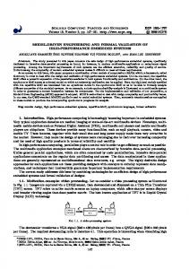
The modern production systems need to be more flexible and re-configurable. For this reason they are built from standardised processing modules as shown in Figure 1. The current trend is to implement control of such systems in a decentralised way, by means of software components that run on distributed programmable control devices. Figure 1

A flexible production cell with an ‘intelligent’ automation system illustrating a machine Plug and Play scenario

When new configurations of production systems are formed from the modular components, the testing becomes a bottleneck for quick commissioning. Formal validation can reduce the time-consuming testing and commissioning phases of system’s development and deployment. As the functionality of such systems is determined by cooperation of entities of heterogeneous domains, for example, mechanical, electric, automation hardware and software, the validation has to take into account the relevant properties from all these domains. The formal modelling and verification techniques, originally created in computer science, were adopted to the area of industrial automation and extensively developed in the past one-two decades. The landmark works, for example, Alur et al. (1990), Clarke et al. (1986) and Sreenivas and Krogh (1991) have set up the general framework and its customisation paths were outlined in a number of subsequent works such as Aygalinc and Denat (1993), De Loor et al. (1997), Hanisch et al. (1997) and Heiner and Menzel (1998). Numerous approaches developed since then differ according to several main criteria, such as, source code-based modelling versus prototyping and code generation, particular programming languages used to describe controllers, particular formalisms used for modelling, closed-loop system representation versus input/output behaviour of the controller. A good survey on the use of formal methods in industrial automation is provided by Bani Younis and Frey (2003).

78

H-M. Hanisch et al.

Thus, a number of test cases have proved that formal modelling can be very helpful for the validation of automation systems by simulation and/or by formal verification of static and dynamic properties. However, despite the activity in the academic community, and even some pioneering attempts of industrial test cases and commercial product development (e.g. ControlBuild Validation of TNI Software), the formal methods have not become a routine tool of control engineers yet. Some of the reasons of that are addressed in this work. The reason to conduct yet another study reported in this paper was the belief that the approach developed by the authors (for more than one decade starting with Rausch and Hanisch (1995)) has a number of features whose combination may make essential difference in applicability for real industrial cases. The cornerstone of this approach is the idea that the models need to be built having in mind that in automation systems the software represents a variable part, while the models of equipment can be reused through the engineering cycle over and over again. Once developed, say by a machine vendor, the models may follow the equipment, enabling the machine users (e.g. system integrators) to validate new configurations of the machines reusing the models of their components. Implementation of this vision, however, requires a more systematic approach to the modelling than that can be seen now, with more emphasis paid on the modelling of plant. Models in most of the formalisms, such as Petri nets or finite automata, lack integrating capabilities: while they may cope well with the modelling of a particular process, building the overall model of a system comprising several processes is difficult. The approach presented in this paper attempts to overcome the weakness of the modelling techniques using the formalisms of Net Condition/Event Systems (NCES), first introduced by Rausch and Hanisch (1995) that added an option of modular thinking to the expressive and analytic power of Petri nets. The modular capabilities have encouraged further development of a systematic approach to the modelling of industrial systems. Supported by the model-checking tools SESA (SESA, 2004), MOSAIC and later iMATCh, the formalism of NCES was used in a number of studies on formal validation of automation systems in process industries and in advanced manufacturing, for example as reported by Hanisch et al. (2000). In the work (Vyatkin 1999), the NCES formalism was used for formal modelling of the new concept for distributed automation function block programming, that later became the IEC61499 standard (IEC61499, 2005). A more comprehensive report on that activity is given by Vyatkin and Hanisch (2003). Along with proving the benefits of NCES, these works have revealed certain limitations, for example, they raised questions of creating nested modular models. The encapsulation of a network of modules inside a module was not carefully worked out so far, although partially the challenges related to the hierarchical modularity concept were faced by Thieme (2002). This paper reports on the comprehensive work started with the development of the ‘extended’ NCES concept by Vyatkin et al. (2003) and forged in course of collaboration in project MOVIDA. The extended NCES was applied for modelling of a number of systems, and a number of new supporting tools have been developed. Together these tools form a new, integrated modelling and verification environment that is supposed to be used directly by engineers that develop control software of automation systems. The results of this work were partially reported by Lobov et al. (2003, 2004) and Vyatkin et al. (2003, 2004).


79

The paper is organised as follows. Section 2 recalls the closed-loop modelling of automation systems. In Section 3, the NCES formalism is introduced and some of its extensions are discussed. Section 4 deals with the systematic modelling of machines and their parts, while Section 5 provides general ideas on the modelling of controllers, which are specified for two programming languages – Flow Charts and Ladder Logic. Section 6 describes the framework of supporting tools and Section 7 illustrates some scenarios of validation by verification using practical industrial-scale examples. The paper is concluded with a discussion of future research plans, acknowledgements and references.

2

Formal methods in automation: application scenarios

2.1 Closed-loop modelling An industrial automation system can be seen as built from two conceptually different parts: controller and plant. The controller is a hardware device driven by software code that performs data processing, communication and decision making, the plant contains the material-handling part of equipment. Figure 2 shows an example of such a control system for a very simple process – filling of the tank with some liquid. The tank has an input valve that controls the liquid supply. Once the tank is filled the valve should be closed. A level sensor (L) indicates the level where the filling should terminate. Figure 2

Example of automated system

Correspondingly, modelling of automation systems can be done in either open-loop or closed-loop way. The open-loop modelling usually is a more economical solution, which bases on the partial model of controller inputs which help to generate the outputs and then verify their correctness. In the closed-loop approach the model of system is composed of two independent components: a model of the object (also known as plant) and a model of the controller, connected in a closed loop by control signals and process data. Both parts are modelled using a common formalism. This approach allows specification of desired/prohibited behaviour of the automation system in terms of the events/statements related to the object rather than in terms of input/output variables. The closed-loop approach is also beneficial in terms of complexity as a feasible model of plant restricts the controller’s input combinations. The model of plant not only generates the inputs of the controller but also receives the outputs and correspondingly modifies its internal state. Certainly the latter approach is more complex as the modelling of uncontrolled reactive behaviour of objects is required. However, its benefits overweight the extra work needed. Both parts of the system (plant and controller) are modelled by NCES modules

80

H-M. Hanisch et al.

with condition signal inputs and outputs. The connection between controller and plant is implemented via logic level signals, which are modelled using condition arcs. Event signals are used in both models of plant and controller but not between them. In the model of plant the events may be used, for example, to model the causal behaviour of sensors influenced from the observed processes. In controllers the event signals model the actions explicitly defined as event-driven (say, event-connected function blocks in IEC1499), as well as a lot of other internal operations: procedure calls, setting/resetting variables, etc. (Figure 3). Figure 3

Closed-loop NCES model of the automated tank filling system

It is worth mentioning that the closed-loop approach to the modelling enables expression of the specifications directly in terms of the machine behaviour (not only I/Os of the controller). The approach allows for a number of application scenarios that can be derived from the diagram in Figure 4. The scenarios include source-code-based modelling of the controller or controller prototyping by a model, as well as formal synthesis of the controller. In all cases, the model of controller is combined with a manually created model of plant. Figure 4

The framework for formal methods use in automation

The prototyping scenario can be less resource-consuming during the validation if compared to the source-code-based model generation as the model of controller may cover only essential issues without implementation details.


3

81

Net condition/event systems

3.1 Basics The formalism of NCES was introduced by Rausch and Hanisch (1995) and further developed through the last decade, in particular by Hanisch and Lüder (1999) according to which a NCES is a place-transition net formally represented by a tuple:

NCES = ( P, T , F , CN , EN , C in , E in , C out , E out , Bc , Be , Cs , Dt , m0 ) where P is a non-empty finite set of places, T is a non-empty finite set of transitions, disjoint with P, F is a subset of ( P × T ) ∪ (T × P ) – the set of flow arcs. CN is the set of condition arcs CN ⊆ ( P × T ) . EN is the set of event arcs EN ⊆ (T × T ). Cin is the set of condition inputs. Ein are the event inputs set, Cout and Eout are conditions and events outputs. Bc is the set of NCES module condition inputs arcs Bc ⊆ (C in × T ), Be is the set of event input arcs Be ⊆ ( E in × T ). Cs is the set of condition output arcs Cs ⊆ (P × E out ) , Dt is the set of event output arcs Dt ⊆ (T × E out ) and m0: P → {0,1} is the initial marking. Figure 5 illustrates the graphical notation of an NCES module. Each module has inputs and outputs of two types: •

condition inputs/outputs carrying state information and

•

event inputs/outputs carrying state transition information.

Figure 5

A module of NCES

Condition input signals as well as event input signals are connected with transitions inside the module. Thus, firing of a transition depends not only on the current marking (as it is the case in Petri nets) but also on the incoming condition and event signals. Incoming condition signals enable/disable a transition by their values in addition to the current marking. Incoming event signals force transitions to fire if they are enabled by marking and by condition signals.

82

H-M. Hanisch et al.

Hence, we get a modelling concept that can represent enabling/disabling of transitions by signals as well as enforcing transitions by signals. More than this, the concept provides a basis for a compositional approach to build larger models from smaller components. ‘Composition’ is performed by ‘gluing’ inputs of one module with outputs of another module as depicted in Figure 6. Figure 6

An example of a modular composition

Result of the composition of two NCES N1 and N2 is an NCES Nc obtained as a union of the components and which can be represented as a new module. Inputs and outputs of the ‘composition’ are unions of the components’ inputs and outputs, except for those which are interconnected to each other, and hereby ‘glued’, that is, substituted by the corresponding condition and event arcs. NCES having no inputs are called Signal/Net Systems (SNS). The model in Figure 6 having modules boundaries removed would be called a SNS. The SNS can be analysed without any additional information about their external environment. The semantics of SNS is defined by the firing rules of transitions. There are several conditions to be fulfilled to enable a transition to fire. First, as it is in ordinary Petri nets, an enabled transition has to have a token concession. That means that all pre-places have to be marked with at least one token. In addition to the flow arcs from places, a transition in SNS may have incoming condition arcs from places and event arcs from other transitions. A transition is enabled by condition signals if all source places of the condition signals are marked by at least one token. The other type of influence on the firing can be described by event signals which come to the transition from some other transitions in the net. Transitions having no incoming event arcs are called spontaneous, otherwise forced. By default presence of at least one non-zero event signal is required to enable transitions by event signals. A forced transition is enabled if it has token concession and it is enabled by condition and event signals. For more rigorous NCES definitions and properties we refer the reader to Starke and Hanisch (1997), Starke et al. (2004) and Vyatkin et al. (2000).

3.2 NCES features for modelling automation systems Thus, the formalism of NCES has the following features: •

it is modular, that is, it provides encapsulation of place/transition models into modules, connected to each other by condition and event arcs

•

it is graphical, that simplifies understanding of the model’s semantic and facilitates application by engineers

Formal validation of intelligent-automated production systems •

it is a distributed state formalism, that helps to cope with the complexity of model-checking, especially when decentralised systems are modelled

•

it is a discrete time formalism, that allows to add new, time dimension to the discrete modelling.

83

In the last decade the automation has been becoming a field of numerous distributed architectures (e.g. IDA, 2002; IEC61499, 2005; PROFInet, 2004), to mention a few. Common in all these is the representation of automation systems as networks of function blocks. Evident similarities between the NCES modelling concept and the advanced trends in distributed control architectures have motivated further development of the NCES formalism that, in particular, was concerned with the definition of model types to simplify encapsulation and reuse of the models. Modelling experiences with NCES so far dealt with control systems of medium complexity. In addition, the modelling was done rather manually. Systematic application of the modelling approach to more complex systems raises many questions on feasibility of some constraints initially introduced in NCES. For example, less restricted rules for interconnections of modules (e.g. allowing for multiple input and output links to a single input element) were considered by Thieme (2002).

3.3 Model type definition in NCES In the presented version of NCES a model has to be encapsulated in a module. A module is defined by its interface and content. The interface contains a model name and names of event and condition inputs and outputs. The content can be either a place-transition model, that is, consist of places, transitions and arcs as described in the previous section (such model types are called basic), or be a network of modules interconnected via event and condition arcs (such models are called complex). Once defined and placed in the library, a module defines a model type. The module name serves as the type identifier. Type instances can be used over and over again in the complex models (strictly speaking, the modules forming the complex models have to be instances of other modules). The extension above makes the NCES ‘compatible’ with other kinds of object-oriented modelling, for example, using Unified Modelling Language (UML). Several works appeared recently on application of object-oriented modelling to machines and production systems (e.g. Bonfè and Fantuzzi, 2003; Thramboulidis, 2001). The UML class diagrams are used in these works to represent the structure of production objects as composed from more elementary ones. That also paves the way to hierarchical models. However, application of UML for formal analysis is difficult as it lacks formality. Thus, the approach presented in this paper bridges the gap between the expression power of UML and the formal semantics of NCES. As a consequence of the above definition a model can have a hierarchical structure as the one presented in Figure 7. The hierarchical structure can be transformed into a plain SNS by instantiation of a model types. Dynamic models of complex objects usually consist of models of their constituent components interconnected by event and condition signals. They may also include an additional model that integrates and coordinates them. Such a ‘master supervisor model’ can also take care about input–output behaviour of the complex model.

84

H-M. Hanisch et al.

Figure 7

4

A hierarchical NCES model

Modelling of automated plants

4.1 Introduction In this section, we will show how the modelling of plant may benefit from the hierarchical model organisation and the reuse opportunities provided by the extended NCES. Thus, common modelling components may be reused in the same model and across different models. Models of the plant and model of the controller are interconnected into the closed loop providing the representation of entire system that consist of the controlled equipment and control device. The combined model is subject for making a judgement about modelled system properties by means of model-checking.

4.2 Systematic methodology Depending on the required accuracy of modelling, the model of plant may include components for each drive, motor, valve, electric relay, sensor, actuator and other elementary pieces of equipment. These component models may be integrated to the complex models of equipment units, such as machine tools, other material processing and storage units and the transportation means. The approach presented in this section extends the ideas of plant modelling of Hanisch and Lüder (2000) and Hanisch et al. (1998). Benefits of the typed modelling are better visible in the following example of object modelling. The automated lifter (product of Flexlink Automation Oy., Finland) as shown in Figure 8 is used in production of electronic components as the system in Figure 1. The lifter can be controlled by two different controllers: an OMRON PLC programmed in ladder logic and Nematron SoftPLC (Lastra, 2000; Nematron Corp., 2001) programmed in Visual Flow Chart language. Though both controllers achieve similar control goals,


85

the internal logic of control algorithms and even the logic of program execution are completely different (cyclically scanned versus sequential). However, both controllers eventually deal with the same object. Figure 8

The lifter, its structure and operation sequence

When the closed-loop plant-controller systems are validated, the model of the lifter can be reused over and over again in connection with models of controllers of different types. The lifter consists of three transporters, one of which is mounted on a vertically moving platform driven by a step motor as schematically represented in Figure 8. The figure also shows sensors (B/S) and actuators (M) of the lifter described as follows. The lifter is composed of three conveyor elements. The pallet is received from the previous module at the lifter’s lower terminal, which is driven by motor M3 and is equipped with B1 sensor that may detect the presence of the pallet. The pallet may be conveyed from the lower terminal to the sledge conveyor that can move vertically between lower and upper terminal (or otherwise it is restricted with the two safety switches S7 and S8). The sledge has B3 sensor that detects a pallet and its belt is driven by motor M1. The upper terminal sensor is B2 and the motor denoted by M2. Besides the conveyors and their sensors and actuators, there is also an operator interface with switches (S1–S5), B5 sensor, which is a safety sensor to detect an obstacle between sledge and terminals. The step motor and the rotary encoder that is used for vertically position the sledge are omitted in Figure 8. The figure does also not show the interface signals (SMEMA) that are used between the lifter and the previous/next module. Each sensor and actuator has a unique name in mechanical/electrical blueprints and software code. The mechanical and electrical drawings with the general description of functionality form the logical point to start plant modelling. The structure of the model type ‘Lifter’ can be represented by means of UML class diagrams as shown in Figure 9. The definition literally says that the object ‘Lifter’ consists of four elements. The loading and unloading one-directional conveyors are identical but turned in opposite directions. The corresponding models are of type Conveyor. The vertically moving platform (an object of type StepMotor) has a moving belt that moves pallets in both directions (modelled as an object of type Conveyor2D). Note that the model in Figure 9 does not define an interface of the lifter, nor dependencies between its constituent parts. These dependencies can be reflected in modular models by event and condition connections between the corresponding modules as exemplified in Figure 10.

86

H-M. Hanisch et al.

Figure 9

Figure 10

Definition of the model type (class) ‘Lifter’ by means of UML class diagrams

A model of Lifter represented as a network of NCES modules

Let us consider the model of a conveyor. In our example, two different types of conveyors are used – capable to move only in one direction, and those moving in both directions. The model of the more complex conveyor can be created based on the simple model using the mechanism of inheritance. The interface of the model type ‘Conveyor’ can be seen in Figure 10. The model itself can be conceptually divided into three elements: Status, Position and Sensor as shown in the class diagram in Figure 11 (left). The Status element of type MovingStatus models the behaviour of the motor that drives the conveyor and converts the logic control signals into one of the states ‘Moving’ or ‘Standing still’ (that corresponds to the one-directional conveyor). Input ‘PRESENT’ indicates if a pallet is present, and input ‘FORCED’ is used to indicate the influence of a neighbour belt on the movement of the pallet. The output condition FW_ST is used by the model of belt position. The structure of the model of the bi-directional conveyor is identical to that of the unidirectional one. The difference is in the module Status that has type MovingStatus2D that inherits the interface properties of the one-directional MovingStatus and extends them with one more input and output for the retracted movement. This is shown in Figure 11(right). All transporters are equipped with a single position sensor indicating the presence of the pallet (fully loaded on the conveyor).

Formal validation of intelligent-automated production systems Figure 11

87

Model type definition of the conveyor and inheritance of the MovingStatus model types

The condition and event flow connections between the submodels constituting the model of the conveyor are represented in Figure 12. Figure 12

Modular view of the model of conveyor

The basic models can be described further in form of NCES modules. Figure 13(a) shows an implementation of the MovingStatus in NCES. The model receives the control signal FWD and transforms it into the state of the belt: place p2 corresponds to the state ‘belt stands still’, place p1 – belt moves and p3 to the state indicating a failure. The belt moves when the control signal FWD is ON, and stops when the signal goes OFF (in the model the negation of the signal FWD goes on). An occurrence of a failure is indicated by an external event that may come from the corresponding model. For example, that can be a non-deterministic model of failures. Note that the model is sensitive to failures only when the belt moves, that is, when the place p1 is marked. It is assumed that the failure can be fixed by an external interaction indicated by the event input RESUME. The model MovingStatus2D for the bi-directional moving belt is shown in Figure 13(b). It models an additional state of backwards moving, and correspondingly has more transitions between the possible states.

88

H-M. Hanisch et al.

Figure 13

Models of the moving status for (a) unidirectional and (b) bidirectional belts

The position of the pallet on the belt can be modelled with different precision. A qualitative model in Figure 14 distinguishes only 3 states of a pallet on the belt: no pallet, pallet on the belt with its front edge between the belt’s ends and pallet’s front edge is beyond the right end of the belt. Figure 14

A qualitative non-timed model of the pallet’s position

A more precise modelling of the position can be done using the timed version of NCES. Let us assume that the belt is 3 units long and the pallet is 2 units long as shown in Figure 15. The speed of the belt is one unit of the length per second. Then it will take three seconds for a pallet to reach the right end of the belt and 2 more seconds to leave the belt completely. Place p1 corresponds to the state ‘No pallet’. When a pallet appears (input condition ‘Present’) and the state of the moving belt is ‘Moving forward’ (indicated by the input condition FWD) then the transition t1 occurs and the token goes to place p2.


89

This place indicates the state ‘Front edge of the pallet is in the interval 1 of the conveyor’. Another reason to transfer to this state is the presence of the input condition ‘Forced’. This condition indicates that the pallet is pushed onto the belt by some external force that maybe another moving belt positioned backwards to this one. This option is modelled by transition t12. In general, moving in this case is slower than if driven by the own motor of the belt. The presented model, however, does not cover with enough precision the case when both forces are present simultaneously. Note that the transition from p1 to p2 (either via t1 or t12) is a qualitative one and does not take time (more precisely has zero delay). Figure 15

Model of the position of the pallet on the conveyor discretised on three intervals

The places p2–p4 correspond to the location of the pallet (again the front edge) in the intervals 1–3, respectively. A transition from interval i to interval i +1 occurs in either case ‘FWD’ and ‘Present’ or ‘Forced’ and ‘Present’. The latter, however, works only till less than the half of the pallet is on the belt – beyond this point the friction force would not let the pallet move driven only by the external force. The moving to the next interval takes 1000 ms if driven by the own motor of the belt or twice as long under the external force. The backward moving from interval I + 1 to interval i occurs if the combination of input conditions ‘RETR’ and ‘Present’ are true. It also takes 1000 ms under assumption that the speed of the moving belt in both directions is the same. Arriving of the pallet to the third interval is indicated by the sensor. This is modelled by two event outputs ‘Sens_ON’ and ‘Sens_OFF’ associated with firing of transitions t8 and t9 or t11, respectively. The sensor goes off when either the front edge of the pallet moves backward to the second interval, or when the back edge of the pallet leaves the belt in forward direction (and the pallet completely disappears from the belt).

90

H-M. Hanisch et al.

This model can represent the state of the pallet on the belt with better precision. However, it has other limitations. In particular, let us consider how the alternative kinds of movement are modelled. A place indicating a position (e.g. p3 indicating interval 2) has several outgoing arcs (p3–t4, p3–t5 and p3–t14) marked with non-zero time delays ([1000, ∞], [1000, ∞], [2000, ∞]). Transitions that are targets of these arcs have condition input signals that represent alternative control signals (RETR, FWD, Forced). Any of the transitions will fire when it is enabled by marking, conditions and time. It is important that all these conditions are mutually orthogonal (alternative) and they never change values within the minimum delay of the place (1000 time units in our case), otherwise the model will not work as intended.

5

Source code based modelling of controllers

5.1 General considerations A model of the controller can be built based on the source code of the control program. Relevant properties of system routines also have to be taken into consideration. The source code based validation gives an additional assurance in the correct behaviour of the system after commissioning. The basics of the modelling of discrete controllers using place-transition formalisms were developed by Hanisch et al. (1997). In general the modelling of controllers can be split into the following sub problems: •

modelling of system routines such as scan cycle

•

modelling of PLC execution is related to the performance of PLC hardware represented by times, instructions execution times, etc.

•

modelling of basic Boolean data and operations

•

modelling of non-Boolean functions.

The use of NCES simplifies the assembling of the model from the components. Besides, such NCES features as event/condition connections closely correspond to the latest trends in controller design methodology presented in new international standard IEC61499.

5.2 Languages for PLC programming 5.2.1 Overview Special industrial programming languages are applied for implementation of the control algorithms. The most of the known programming languages in the field were standardised in IEC 61131-3 in 1993 (IEC 61131, 1993). The standard includes four programming languages: Instruction List (IL), Function Block Diagrams (FBD), Ladder Diagrams (LD) and Structured Text (ST) and a common element Sequential Function Chart (SFC) that serves for program organisation into logical steps and expressing the transitions between the steps. Despite the successful standardisation of PLC programming, there is a number of vendor specific programming approaches that have not been included in IEC61131-3,


91

although they are quite popular in certain application areas. In this paper we exemplify our approach on two specimens: ladder logic language that is an Omron implementation and flowchart language that of Nematron Corp. (2001).

5.2.2 Ladder logic LD is a widely used industrial programming language. It resembles relay diagrams from the times when the control system were built as hardware circuits from relays. Nowadays LD programs may contain complex mathematical functions executed on PLC hardware. A single-rack LD program is shown on the left in Figure 16. IX_Tank_Full variable represents a PLC input signal coming from the level sensor of the tank L. QX_Valve_In is PLC output that controls the input valve of the tank. A representation of both input/output variables in NCES is defined in Figure 23. Figure 16

Tank control program

The program is written for Omron CPM1A PLC. The Omron control software development tool (CX-Programmer) is made to support a set of dozens of Omron PLCs. The same environment and the same programming language is used for each controller, the difference may be in the amount of supported functions. One of the features of CX-Programmer software is an ability to save project’s data in a text file. The file would contain all possible data related to the project and controller.

5.2.3 Flowcharts The flowcharting was used years ago for the programmers for prototyping and documenting of programs. Herman H. Goldstine and John von Neumann developed flowcharting in 1947 as a means of representing a computer algorithm at a level higher than that of machine language. Flowcharting as a means of programming in industrial automation has emerged about a decade ago. There are several implementations known, mainly for PC-based control devices called SoftPLCs. One of such SoftPLC products namely OpenControl (OC) of Nematron Corporation uses Visual Flowchart Language (VFL) as a high-level programming language (Nematron Corp., 2001). A flowchart-programmed automation project may contain one or more flowcharts. A flowchart (as exemplified in Figure 17) may consist of a set of the blocks, which represent the program behaviour.

92

H-M. Hanisch et al.

Figure 17

Flowchart and its basic components

VFL has two basic types of elements. These are decision blocks and process blocks. The process blocks represent operations on data. They may contain several commands that can perform calculations, data modification and communication operations in the PLC program. Program branching and cycling is mainly organised by decision blocks (If-Then-Else, While Do and Repeat Until). The Boolean expressions of the blocks are evaluated in order to define the program execution path. Branches of the decision blocks may contain any other blocks. The control of program execution path can be done by the pairs of the Goto and Goto Label blocks. An essential program organisation unit of the Visual Flowchart Language is a subchart. A subchart can be seen as a procedure, which can be called or addressed by a Subchart Call block. Subcharts can be described by the same blocks as a flowchart. Each flowchart can be considered as a separate task. During the flowchart evaluation phase of the scan cycle, each flowchart gets its execution time. The flowchart runs till it solves all logic from the first block till the last block in the flowchart or till it meets the situation where the execution has to be yielded to the next task.

5.3 Modelling of system routines in PLCs Precise modelling of automation systems requires to take in account quite low level details of the control program execution in a PLC. The PLC programs are executed in a cyclic way. One cycle consists of the following phases: first the inputs are read, then the program logic is executed and then the outputs are written. Figure 18 depicts a NCES skeleton for a PLC model. Place p1 holds a token representing the initial state of the PLC execution, if the PLC program is enabled (condition input to the t1 transition) the cycle is started by the update of outputs and acquisition of input values. The firing of t1 transition generates these events. When a token is placed to p2, it resides there until a signal notifying about the change in the system enables transition t2. The monitoring of the changes in the systems is needed in order to not start a new PLC cycle unless something has changed in the system.

Formal validation of intelligent-automated production systems Figure 18

93

PLC model skeleton

The state of the NCES model is distributed and is defined by the marking of all places. Additionally to the marking, the state is characterised by the time stamp, for example, the time the certain state (marking) is valid. Thus the two states representing the same marking but holding different times are different states. A special module that monitors the change in the system has to be added to the model (Figure 19). The module has two event inputs for retrieving information about any change of the PLC program variables during the scan cycle. It does not make sense to run the model over the new scan-cycles if the markings in the model remain unchanged, that is, when nothing would change during the next scan. The marking may change in the model of the plant or if the time dependent transition fires in a timer NCES module in the model of controller. Figure 19

Change monitoring NCES module

5.4 Modelling of system routines in SoftPLCs Following the traditions of common PLCs, the SoftPLCs implement the scan based approach of program execution. The PLC execution cycle has three main phases: at the first phase the inputs are read then the logic is evaluated, and at the third phase of the cycle the outputs are updated. The cycle is executed over and over again. In SoftPLCs this cycle is placed into HyperKernel (HK) execution, which is interleaved with the execution of other OS tasks. The HK itself can be considered as a small OS responsible for time scheduling between the control tasks.

94

H-M. Hanisch et al.

Figure 20 illustrates the execution cycles of the SoftPLC. Steps numbered from one to four correspond to the traditional PLC cycle phases. These phases are enabled within the time frame allocated to the HK execution. In our case time is shared between HK and Windows NT in equal slots – both are getting 250 ms (this value is adjustable) of execution time. If the cycle 1-2-3-4 has been already started when the HK time has expired the HK yields the execution control to Windows. After the OS execution is over, the PLC scan cycle is resumed from the place where the HK yielded the control. The switch between HK and OS can be represented by the NCES shown in Figure 21. Figure 20

SoftPLC scan cycle

Figure 21

NT/HK switch NCES module

Place p1 can be considered as the representation of the state of HK execution time. The condition arc coming out of the place to condition output ‘ENABLED’ is the enabling signal for PLC program execution. Transition t1 is forced to fire after 250 ms have expired. In the figure, this behaviour is expressed by the time interval attached to the


95

flow arc (p1, t1). When place p2 holds a token the ‘NOT_ENABLED’ condition output is activated. And again, transition t2 is forced to fire after 250 ms. Figure 22 shows the NCES module of the scan-cycle model which models the time sharing process between several flowchart tasks. Figure 22

Model of the flowcharts’ scheduler

The places {p1, p3, …, pN} denote the situations when the particular flowchart is being evaluated. Each place has condition output arc that is intend to be interconnected with the corresponding flowchart. The condition inputs labelled ‘ENABLED’ and ‘NOT ENABLED’ are coming from NT/HK switch module described previously (Figure 21). Some of the places denoted as {p11, p21, …, pN1} hold the token during the OS execution time. The token is considered to be moved to the place of {p11, p21, … , pN1} from the corresponding place of {p1, p2, …, pN} in the situation when the ‘NOT ENABLED’ signal is coming from the NT/HK Switch module. Two event outputs labelled as ‘writeO’ and ‘readI’ are provided for activating input/output sampling phases of the scan cycle. When of the places {p1, p2, …, pN} holds a token the corresponding flowchart gets its execution time. The enabling signal is sent to the flowchart by the condition output arc. The condition outputs are labelled {‘ENABLED1’, ‘ENABLED2’, … , ‘ENABLEDN’}. The event inputs labelled {‘YIELD1’, ‘YIELD2’, … , ‘YIELDN’} are coming from the NCES modules representing flowcharts, through these the scan cycle is notified that the next flowchart has to get its execution time or, if the flowchart is the last on the list, YIELDN notifies that the values of output variables can be written now to the peripheral hardware. The NCES modules representing the flowcharts are in a closed-loop connection with the scan cycle representing NCES module through the ENABLEDX – YIELDX input–output pair, where the flowchart is coming in between. Combining two blocks given in Figures 21 and 22 would give a framework for the SoftPLC scan-based cycle behaviour. What is missing so far is the PLC data and program models that are introduced in the following sections.

5.5 Modelling of data PLC programs deal mainly with Boolean data. We model Boolean input and output variables in the way similar to the one suggested by Hanisch et al. (1997) and Hanisch and Lüder (2002). In addition to the representation of a Boolean variable defined in that paper an extra change event output is added to the corresponding NCES module (Figure 23).

96

H-M. Hanisch et al.

Figure 23

Boolean input, Boolean output and Boolean output module with the temporal value (Lobov, 2004)

The event input of the input’s NCES module is provided by the NCES scan cycle module (Figure 20) labelled as ‘readI’. The condition output arcs coming out of p1 (VarON) and p2 (VarOFF) places provide the recipient parts of the flowchart model with the appropriate values of the input variable. The Output model using NCES has a difference as compared to the input module. There is no triggering even input ‘update’. Instead, the output model has two event inputs, which allow the flowchart model NCES to set or reset the variable used by it. The condition output arcs of p1 (VarON) and p2 (VarOFF) places provide signals to plant model. Non-Boolean (e.g. integer) values still can be efficiently handled by utilisation of discrete thresholds.

6

Tool framework

6.1 Framework overview To facilitate the use of NCES by engineers, the formalism is supported by tools and methodologies as follows: •

graphical editors provide full graphical authoring and editing of the models

•

iMATCh – an integrated tool that contains a model builder (assembler), a translator to the flat format for subsequent model-checking, interfaces to several model-checkers, and the means for analysis of scenarios (e.g. their visualisation in the form of state/time diagrams) or even system simulation along the selected scenarios


the model checker SESA allows for efficient model-checking of fairly complex systems (millions of discrete states)

•

the application methodologies are represented as libraries of standard model elements and by the web-based documentation.

97

6.2 Model creation and editing Formalisms having a graphical notation have clear advantages compared to purely analytic ones. To enjoy the benefits in full scale the model authoring and maintenance have to be supported in a visual intuitive way. Currently the NCES modelling is supported by the editor developed at Martin Luther University of Halle-Wittenberg (Figure 24). Figure 24

Screen-shots of the NCES editor

The editor provides full graphical authoring and editing of the models. The need to reuse models has pushed the development of an open XML-based data format for basic and composite NCES models. The editor uses the XML-based format for storing basic and composite NCES models. The data format of composite model blocks was intentionally made identical with that of IEC61499 function blocks. Thanks to the commonality the library of models can be accessed also by the function block tool FBDK (2005).

98

H-M. Hanisch et al.

The user fills the library of model types by creating the types from basic or complex NCES modules. The ‘typed’ approach facilitates the reuse of previously developed model components. The editor allows manual assembly of NCES modules into more complex composite models. The model of a controller can be generated by the MOVIDA NCES Generator (Figure 25). The generator inputs a controller represented as a textual file of Omron Ladder Diagram project, converts it to NCES and saves the data in XML-based format. This illustrates how the openness and self-explanatory XML representation simplifies the development of the tools that may work with NCES. Figure 25

Screen shot of the MOVIDA NCES generator

6.3 Integrated tools for model assembly and analysis The integrated environment for Model Assembly (iMATCh) inputs the model type files given in XML and is capable of: •

Assembling of a composite, hierarchically organised model from modules contained in different libraries of model types. The component model types are instantiated into NCES modules.

•

Translating the model into a ‘flat’ NCES with the through numbering of places and transitions. The inter-module connections are converted into event and condition arcs between places and transitions. Thus the module boundaries are removed and the model-checking tools can be applied. In particular, the translator generates files in the input format of SESA model checker.


iMATCh can prove specifications in the form of first order predicates or can pass the temporal logic formulae to SESA model checker. The internal model checker of iMATCh generates the reachability graph for the model, either completely or dynamically while it checks the formula. It can also import a reachability graph generated by SESA and visualise it.

•

Once a state with particular properties is found in the reachability space, iMATCh can visualise a path from initial (or any other state) to the found one. The visualisation is done in form of state-time diagram for a selected set of system variables (both from plant and controller). A user can select between different views and see the model in each state. The visualisation options proved to be very useful in practical verification.

99

The iMATCh tool is still under development and its trial version can be requested from [email protected]. (Figure 26). Figure 26

7

iMATCh tool visualising a reachability graph and a path in that graph by state-time diagrams

Validation

The validation of automation systems modelled by NCES can be performed by simulation and formal verification via model checking. The simulation usually can follow a limited number of scenarios in the system’s behaviour while the potential flaws can be in those paths left out unvisited. The multiple scenarios may result from the influence of some unpredictable factors, such as variable

100

H-M. Hanisch et al.

durations of some operations, communication delays, malfunctions, etc. In contrast, the model-checking explores all the existing scenarios. The verification consists in proving specifications with respect to the dynamic behaviour of the model. The specifications can be given either in form of second order predicates, or in form of temporal logic expressions, for example in Computational Tree Logic (CTL). The basic terms of these expressions in most cases are the ‘values’ of inputs and outputs (either of plant or controller) or, literally, the marking of the corresponding NCES modules modelling the data variables. As the hierarchical NCES model is converted into a flat SNS model this provides the through place/transition numbering, and these numbers are used as references to the values. In case of the lifter the following groups of specifications were of the primary interest: •

Avoidance of potentially dangerous situations that may lead to a breakdown of the lifter or to damage of the product being transferred by the lifter. Example: when used in manufacturing of precise electronic components, such as hard drives, the lifter must never allow the situations when the pallet leans or jumps. Such problem can be caused by inexact synchronisation of conveyors’ levels, which, in turn, may be a result of wrong synchronisation of control programs.

•

Robustness of the system in case of malfunctions of some sensors.

•

The control programs in VFL are branching. Formal verification helps to prove that the response time is never exceeded in any feasible I/O combination in any branch.

•

Avoidance of deadlocks or ‘dynamic traps’ that may result from wrong synchronisation of operations.

•

Presence of certain ‘checkpoints’ in any possible scenario of behaviour that guarantees all necessary operations have been applied to the product in any circumstances.

Table 1 provides some examples of the formalisation of specification of system requirements. The first column in the table gives a logical proposition formula and expresses the mapping of the local labels in the NCES modules to the global SNS label (given in parenthesis). The second column provides a description of formula arguments given in the first column. The last column contains the case description in a natural language. The long names of’ arguments in the formulae are due to the hierarchy of the modules and the places coming at the lowest level. For instance, ‘Controller._M1DIVIDECW.p4’ is interpreted as place p4 at M1DIVIDECW module (represents the motor of the sledge run clockwise) in the controller module. The requirements specifications given in Table 1 were simplified from the real ones for illustrative purposes, more extensive formulae can be found by Lobov (2004). Once the requirements are defined, the model-checking can take place in the reachability space of the system’s model which for the model of the lifter encountered 59,479 states.

Formal validation of intelligent-automated production systems Table 1

List of specifications

101

102

H-M. Hanisch et al.

Let us consider verification of each formula in more details: 1

‘p213 AND p249’ when evaluated in iMATCH fulfils in no states. That means the controller never turns the motor of the sledge to run into both directions, which could have lead to the physical damage of the motor.

2

Checking of the second formula ‘p472 AND (p213 OR p249)’ gives a set of states for which it is true. Thus, there are states where the lifter is in the middle of its vertical move and the sledge motor is running in either one direction or another. The next step in analysis is to identify the reason. The first step is to define in what direction the motor is running (loading – p213, unloading – p249) or both. This is can be identified by two separate formulae: ‘p472 AND p213’ and ‘p472 AND p249’. Checking both formulae has given the result that only ‘p472 AND p213’ is TRUE and has a number of states in the reachability graph. Furthermore, the direction of motion may be defined by ‘p205 AND p472 AND p213’, where p205 represents upward motion. The formula is false if there is p221 (downward motion) instead of p205. The direction of the vertical and conveyor belt motion is therefore identified. Now, we know that the motor of the sledge runs at the lower terminal level to retrieve the pallet from the terminal. The next step is to find out where the pallet is located. There are several possibilities: a

Plant.Sledge_Conv.Sensor.p2 (p515) – on the sledge

b

Plant.Sledge_Conv.Position.p10 (p529) – the pallet is not on the sledge

c

Plant.Low_Conv.Sensor.p2 (p503) – the pallet is at the lower terminal

We checked the formula ‘p472 AND p213 AND p205 AND p515’ and it is fulfilled in no states. This means that the sensor does not detect the pallet. Checking the ‘p205 AND p472 AND p213 AND p529’ formula finds the same states in the reachability graph as the initial formula ‘p205 AND p472 AND p213’, which means there is no pallet on the sledge at all. Formula ‘p205 AND p472 AND p213 AND p529 AND p503’ again fulfils in the same states. This situation may be interpreted as follows: The pallet is stuck at the lower terminal and has not been transmitted to the sledge. After some timeout for receiving the pallet and without getting it, the lifter starts upward motion while the sledge conveyor continues running. Further investigation shows that the low terminal motor is running as well (Plant.Low_Conv.Status.p1 (p499)), but the pallet remains at the lower terminal (the formula ‘p205 AND p472 AND p213 AND p499 AND p510 AND p503’ gives the same states in the reachability graph). Furthermore, this situation is not found for the sledge in the upper terminal position (Plant.Vertical.Vertical. p3 (p473): checking of the following formula ‘p205 AND p473 AND p213’ gives no states found). This error reveals an uncontrollable object’s property when nothing can be done by controller to resolve it. If this situation were to occur with the real lifter the operating personnel would be required to resolve it and reset the lifter.


103

However, the reason why the controller commands to move up while the loading operation of the sledge is not complete is interesting, but not the primary goal. The primary goal is the conclusion that there were no states found in which the pallet has been successfully loaded onto the sledge (p515), the lifter is half way (p472) driving up (p205) and the sledge motor is running (p213) (‘p515 AND p472 AND p205 AND p213’ checking gives no states found). This situation is one of such type which would not be detected by the common testing. 3

The next formula represents the situation when the sledge motor is running to download the pallet while the lifter is at the upper terminal level where the pallet should be unloaded ‘p473 AND p213’. Checking this simple request gives no states found in reachability graph. It is therefore possible to conclude that the sledge conveyor belt will not run to the wrong direction at the upper terminal level.

4

This formula describes a situation opposite to the previous one: ‘p471 AND p249’. The sledge conveyor is running to unload the pallet at the lower terminal level. Checking of the formula also returns a false result meaning that no such states exist in the reachability graph.

5

Place p503, p515 and p486 model TRUE value of the pallet sensors of the low conveyor, sledge conveyor and upper conveyor, respectively. Checking if any of these places ever holds a token gives an affirmative answer. In this example, we may highlight one of the advantages in applying CTL. The CTL formula ‘E[E[EF m(p503) = 1 U EF m(p515) = 1] U EF m(p486) = 1]’ represents the case when a path exists in the reachability graph where first the low terminal sensor detects a pallet, then the sledge terminal sensor detects a pallet and finally the upper terminal sensor detects a pallet. This is an example of checkpoint rule, proving which we may conclude that the lifter is able to transfer a pallet through it.

The described example may give an idea how the validation routine may look like. The models of the lifter are available in the internet for download (Lobov, 2004). The reader may try to evaluate them by SESA model checker that is also available for download at (SESA, 2004). The overall model had three hierarchy levels and after assembly from modules encountered 571 places and 828 transitions. However, the model-checking of the normal behaviour (without modelling malfunctions in sensors) resulted in a reachability space not exceeding 60,000 states which was generated on a usual laptop less than in a minute. This result reflects the efficiency of distributed state modelling with NCES. The expected state space for the production line shown in Figure1 could be well below a million states which is a very feasible size for the model checking with SESA. Besides the possibility to verify or falsify certain properties of the system, another important advantage is that the method may be applied in absence of physical controller and physical plant. Consider the following scenario: the manufacturing line where conveyor modules, lifters, workstations, robotic cells, etc., are being installed. Mechanical and electrical engineers do installations and tests of the equipments. The time for project runs out, the deadline is approaching, but the control engineer had no chance to test the line, since the physical equipment is not ready yet. In this situation

104

H-M. Hanisch et al.

the application of this method (model-based validation with the model of controller derived from the source code) may provide an environment for independent development of control, while the physical plant is being set up. More details on the practical verification experiences with NCES and the tool framework can be found by Lobov (2004).

8

Conclusion

The reported work convinced us that the efficient reuse of model elements makes a difference in the applicability of formal verification for practical control engineering. The qualitative improvement of the reuse was achieved by the typed modular model organisation. Of special importance was explicit modelling of plant’s structure and dynamics. The integrated model development, checking and analysis achieved by the tool framework ensured further benefits of the approach. Currently, we are working on extending the framework in order to facilitate the development of the models of plant. The recent success of UML as means of model-based system engineering has attracted attention to UML as to the formal modelling formalism also in industrial automation. For example, the works (Bonfè and Fantuzzi, 2003; Takatsuka and Tomita, 2002) present first attempts to this end. The ideas presented in this paper will serve as the basis of an extended modular modelling paradigm combining the object-oriented typed modelling (of the mainstream UML) with the benefits of modular place-transition nets. There is work in progress on further integration of NCES with higher-level UML models being conducted both in the Universities of Halle (Germany) and Tampere (Finland) that extends the results presented in this paper. The conversion of UML state charts defining the dynamics of models into the corresponding NCES models will be the subject of future research. Though the UML support is not integrated to the tool framework as described in the paper, however, the similarity between NCES and IEC61499 function blocks allow for using the CORFU environment (Thramboulidis, 2002) in connection with Rational Rose in order to define the model’s structure and interfaces and convert them to the form of interconnected NCES modules.

Acknowledgements The work was partially supported by MOVIDA-1, a project funded by the National Technology Agency in Finland – TEKES and Deutsche Forschungsgemeinschaft under reference Ha 1886/12-2.

References Alur, R., Courcoubeitis, C. and Dill, D.L. (1990) ‘Model checking for real-times’, Proceedings of the Fifth Annual IEEE Symposium on Logics in Computer Science, Philadephia. Analysing Signal-Nets with SESA (2004) Available at: http://www.informatik.hu-berlin.de/ lehrstuehle/automaten/sesa/.


105

Aygalinc, P. and Denat, J.P. (1993) ‘Validation of functional Grafcet models and performance evaluation of the associated systems using Petri nets’, Automatic Control Production Systems A.P.I.I., Vol. 27, pp.81–93. Bani Younis, M. and Frey, G. (2003) ‘Formalization of existing PLC programs: a survey’, Proceedings of Computing Engineering in Systems Applications, Lille, France. Bonfè, M. and Fantuzzi, C. (2003) ‘Design and verification of industrial logic controllers with UML and state charts’, IEEE Conference on Control Application, 23–25 June, Istanbul, Turkey. Clarke, E., Emerson, E.A. and Sista, A.P. (1986) ‘Automatic verification of finite state concurrent systems using temporal logic’, ACM Transactions on Programming Languages and Systems, Vol. 8, pp.244–263. De Loor, Zaytoon, P.J. and Villerman-Lecolier, G. (1997) ‘Abstraction and heuristics for the validation Grafcet controlled systems’, European Journal of Automation, Vol. 31, pp.561–580. FBDK – Function Block Development Kit (2005) Available at: www.holobloc.org, visited in June. Hanisch, H-M. and Lüder, A. (1999) ‘Modular modelling of closed-loop systems’, Colloquium on Petri Net Technologies for Modelling Communication Based Systems, Proceedings, Berlin, Germany, 21–22, October pp.103–126. Hanisch, H-M. and Lüder, A. (2000) ‘Modular modeling of closed-loop systems’, Colloquium on Petri Net Technologies for Modeling Communication Based Systems, Proceedings, Berlin, Germany, pp.103–126. Hanisch, H-M., et al. (1997) ‘Modelling of PLC behaviour by means of timed net condition/event systems’, Sixth International Conference on Emerging Technologies and Factory Automation, Los Angeles, USA. Hanisch, H-M., Lüder, A. and Thieme, J. (1998) ‘A modular plant modelling technique and related controller synthesis problems’, IEEE International Conference on Systems, Man, and Cybernetics, October, Vol. 1, pp.686–691. Hanisch, H-M., Pannier, T., Peter, D., Roch, S. and Starke, P. (2000) ‘Modelling and verification of a modular lever crossing controller design’, Automatisierungstechnik, Vol. 48. Heiner, M. and Menzel, T. (1998) ‘Instruction list verification using a Petri net semantics’, IEEE International Conference on Systems, Man, and Cybernetics, Vol. 1, pp.716–721. IDA – Interface for Distributed Automation (2002) Available at: www.ida-group.org. IEC61499 (2005) Function Blocks for Industrial Process Measurement and Control Systems, Publicly Available Specification, International Electrotechnical Commission, Technical Communication 65, Working Group 6, Geneva. International Standard IEC 1131-3 (1993) Programmable Controllers – Part 3, International Electrotechnical Commission, Geneva, Switzerland. Lastra, J.L.M. (2000) ‘Evaluation of new open control systems for light assembly applications’, MSc Thesis, Tampere University of Technology. Lobov, A. (2004) An approach to the formal verification of automated manufacturing systems with programmable control, MSc Thesis, Tampere University of Technology, April, Available at: http://www.pe.tut.fi/movida/LobovThesis/. Lobov, A., Lastra, J.L.M., Tuokko, R., and Vyatkin, V. (2003) ‘Methodology for modelling visual flowchart control programs using Net Condition/Event Systems formalism in distributed environments’, IEEE Conference on Emerging Technologies in Factory Automation (ETFA’03), Proceedings, Lisbon, September. Lobov, A., Lastra, J.L.M., Tuokko, R., and Vyatkin, V. (2004) ‘Modelling and verification of PLC-based systems programmed with ladder diagrams’, INCOM’2004, Proceedings, Salvador, Brazil, April. Nematron Corp. (2001) ‘OpenControl: about open architecture’, Available at: http: www.nematron.com/OpenControl/oc_architecture.shtml, September.

106

H-M. Hanisch et al.

PROFInet – project of Profibus User Organization (2004) Available at: http://www.profibus.com. Rausch, M. and Hanisch, H-M. (1995) ‘Net condition/event systems with multiple condition outputs’, Symposium on Emerging Technologies and Factory Automation, Proceedings, INRA/IEEE, Paris, France, October, Vol. 1, pp.592–600. Sreenivas, R.S. and Krogh, B.H. (1991) ‘On condition/event systems with discrete state realizations’, Discrete Event Dynamic Systems: Theory and Applications, Vol. 2, No. 1, pp.209–236. Starke, P.H. and Hanisch, H-M. (1997) ‘Analysing of signal/event nets’, Proceedings of the Sixth IEEE International Conference on Emerging Technologies and Factory Automation ETFA-97, Los Angeles, USA, September, pp.253–257. Starke, P., Roch, S., Schmidt, K., Hanisch, H-M. and Lüder, A. (2004) ‘Analysing signal-event systems’, Technical Report, Humboldt Universitat zu Berlin, Institut für Informatik, Available at: http: www.informatik.hu-berlin.de/lehrstuehle/automaten/tools/, July. Takatsuka, K. and Tomita, S. ‘On modelling and an algorithm for verifying behaviour of discrete parallel production system’, PSE2002ASIA. Thieme, J. (2002) Symbolische Erreichbarskeitanalyse und automatische Implementierung struktuirter, zeitbewerter Steuerungsmodelle, Dissertation zur Erlagung des Grades Dr.-Ing., Berlin: Logos Verl. Thramboulidis, K. (2001) ‘Using UML for the development of distributed industrial process measurement and control systems’, IEEE Conference on Control Applications (CCA), September, Mexico. Thramboulidis, K. (2002) ‘Development of distributed industrial control applications: the CORFU framework’, Fourth IEEE International Workshop on Factory Communication Systems, August, Vasteras, Sweden. Vyatkin, V. and Hanisch, H-M. (1999) ‘A modelling approach for verification of IEC1499 function blocks using Net Condition/Event Systems’, IEEE Conference on Emerging Technologies in Factory Automation (ETFA'99), Proceedings, Barcelona, Spain, September, pp.261–270. Vyatkin, V. and Hanisch, H-M. (2003) ‘Verification of distributed control systems in intelligent manufacturing’, Journal of Intelligent Manufacturing, Special issue on Internet Based Modelling in Intelligent Manufacturing, Vol. 14, No. 1, pp.123–136. Vyatkin, V., Hanisch, H-M. and Bouzon, G. (2004) ‘Open object-oriented validation framework for modular industrial automation systems’, INCOM’2004, Proceedings, Salvador, Brazil, April. Vyatkin, V., Hanisch, H-M. and Pfeiffer, T. (2003) ‘Modular typed formalism for systematic modelling of automation systems’, First IEEE Conference on Industrial Informatics (INDIN’03), Proceedings, Banff, Canada, August. Vyatkin, V., Hanisch, H-M., Starke, P. and Roch, S. (2000) ‘Formalisms for verification of discrete control applications on example of IEC1499 function blocks’, Conference ‘Verteilte Automatisierung’ (Distributed Automation), Proceedings, Magdeburg, Germany, March, pp.72–79.