Formal Verification of Distributed Dynamic Thermal Management

Formal Verification of Distributed Dynamic Thermal Management ∗ School

Muhammad Ismail∗ , Osman Hasan∗ , Thomas Ebi† , Muhammad Shafique† , Jörg Henkel† of Electrical Engineering and Computer Science, National University of Sciences and Technology, Islamabad, Pakistan † Chair for Embedded Systems (CES), Karlsruhe Institute of Technology (KIT), Germany Email: {10mseemismail, osman.hasan}@seecs.nust.edu.pk; {thomas.ebi, muhammad.shafique, henkel}@kit.edu

Abstract—Simulation is the state-of-the-art analysis technique for distributed thermal management schemes. Due to the numerous parameters involved and the distributed nature of these schemes, such non-exhaustive verification may fail to catch functional bugs in the algorithm or may report misleading performance characteristics. To overcome these limitations, we propose a methodology to perform formal verification of distributed dynamic thermal management for many-core systems. The proposed methodology is based on the SPIN model checker and the Lamport timestamps algorithm. Our methodology allows specification and verification of both functional and timing properties in a distributed many-core system. In order to illustrate the applicability and benefits of our methodology, we perform a case study on a state-of-the-art agent-based distributed thermal management scheme.

I.

I NTRODUCTION AND R ELATED W ORK

As the semiconductor industry moves towards smaller technology nodes, elevated temperatures resulting from the increased power densities are becoming a growing concern [11]. High temperatures aggravate reliability threats like aging [11], [12] and soft errors [3], [9], [21]. In fact, Dynamic Thermal management (DTM) of distributed nature has been identified as one the key reliability challenges in the ITRS roadmap [14]. At the same time, the growing integration density is paving the way for future many-core systems consisting of hundreds and even thousands of cores on a single chip [14], [24]. From a thermal management perspective, these systems bring both new opportunities as well as new challenges. For one, whereas DTM in single-core systems is largely limited to Dynamic Voltage and Frequency Scaling (DVFS), many-core systems present the possibility for spreading power consumption in order to balance temperature over a larger area through the mechanism of task migration. However, the increased problem space related to the large number of cores makes the complexity of DTM grow considerably. Traditionally, DTM decisions have been made using centralized approaches with global knowledge. These, however, quickly become infeasible due to lack of scalability when entering the many-core era [7], [8], [22], [24]. As a result, distributed thermal management schemes have emerged [5], [7], [8], [10] which tackle the complexity and scalability issues of many-core DTM by transforming the problem space from a global one to many smaller regional ones which can exploit locality when making DTM decisions. For a distributed DTM scheme to achieve the same quality as is possible from one using global knowledge, however, it becomes necessary for there to be an exchange of state information across regions in order to negotiate a near-optimal system state configuration [7].

The choice of tuning parameters for this negotiation has been identified as a critical issue in ensuring a stable system [15]. Up until now these distributed DTM schemes have been exclusively analyzed using either simulations or running on real systems. However, due to the non-exhaustive nature of simulation, such analysis alone is not enough to account for and guarantee stability in all possible system configurations. Especially when considering many-core systems, the number of different configurations, e.g., task-to-core mappings, grows exponentially with the number of cores. Even if some corner cases can be specifically targeted, there is no proof that these represent a worst-case scenario, and it is never possible to consider or even foresee all corner cases. Moreover, using simulation we may show that for a given set of tasks and cores, a small number of mappings result in localized minima. However, in distributed DTM approaches this actually means that a local region of cores may be successfully applying DTM from their point of view although from the global view temperatures are really maximal. Thus, simulation based analysis cannot be considered complete and often results in missing critical bugs, which in turn may lead to delays in deployment of DTM schemes as happened in the case of Foxton DTM that was designed for the Montecito chip [6]. The above mentioned limitations can be overcome by using model checking [4] for the analysis of distributed DTM. The main principle behind model checking is to construct a computer based mathematical model of the given system in the form of an automata or state-space and automatically verify, within a computer, that this model meets rigorous specifications of intended behavior. Due to its mathematical nature, 100% completeness and soundness of the analysis can be guaranteed [2]. Moreover, the ability to provide counter examples in case of failures and the automatic nature of model checking makes it a more preferable choice for industrial usage as compared to the other mainstream formal verification approaches like theorem proving. Model checking has been successfully used for analyzing some unicore DTM schemes (e.g., [19], [23]). Similarly, probabilistic model checking of a DTM for multicore architectures is presented in [18]. This work conducted a probabilistic analysis of frequency effects through DVFS, time and power spent over budget along with an estimate of required verification efforts. In order to raise the level of formally verifying complex DTM schemes, statistical model checking of power gating schemes has been recently reported [16]. However, to the best of our knowledge, so far no formal verification method, including model checking, has been used for the verification of

a distributed DTM for many-core systems. This paper intends to fill this gap and proposes a methodology for the functional and timing verification of distributed DTM schemes. A. Our Novel Contributions and Concept Overview We present a novel methodology for formal verification of distributed DTM schemes in many-core systems. The key idea is to leverage the SPIN model checker [13] (an open source tool for the formal verification of distributed software systems) and Lamport timestamps [17] (a technique that enables to determine the order of events in a distributed system execution). Our methodology allows the designer to formally model or specify the behavior of distributed DTM schemes in the PROcess MEta LAnguage (PROMELA). These models are then verified to exhibit the desired functional properties using the SPIN model checker as it directly accepts PROMELA models. Our methodology introduces the Lamport timestamps algorithm in the PROMELA model of the given distributed DTM scheme to facilitate the verification of timing properties via the SPIN model checker. In order to illustrate the effectiveness of our methodology, we perform a case study on the the formal verification of a state-of-the-art agent-based distributed DTM scheme, namely Thermal-aware Agent-based Power Economy (TAPE) [7]. The main reason behind the choice of TAPE for this case study is that it is highly scalable while still achieving comparable results to centralized DTM approaches which operate on global system knowledge like PDTM [25] and HRTM [20]. Paper Organization: The rest of the paper is organized as follows: Section II provides an overview of model checking and SPIN to aid the understanding of the rest of the paper. The proposed methodology is presented in Section III. This is followed by the formal modeling and verification of the TAPE algorithm in Section IV. Formal verification results are discussed in V. Finally, Section VI concludes the paper. II.

P RELIMINARIES

A. Model Checking Model checking [4] is primarily used as the verification technique for reactive systems, i.e., systems whose behavior is dependent on time and their environment, like controllers of digital circuits and communication protocols. The inputs to a model checker include the finite-state model of the system that needs to be analyzed along with the intended system properties, which are expressed in temporal logic. The model checker automatically and exhaustively verifies if the properties hold for the given system while providing an error trace in case of a failing property. The state-space of a system can be very large, or sometimes even infinite. Thus, it becomes computationally impossible to explore the entire state-space with limited resources of time and memory. This problem, termed as state-space explosion, is usually resolved by developing abstract, less complex, models of the system. Moreover, many efficient techniques, like symbolic and bounded model checking, have been proposed to alleviate the memory and computation requirements of model checking. B. SPIN Model Checker SPIN model checker [13], developed by Bell Labs, is a widely used formal verification tool for analyzing distributed

and concurrent software systems. The system that needs to be verified is expressed in a high-level language PROMELA, which is based on Dijkstra’s guarded command language and has a syntax that is quite similar to the C programming language. The behavior of the given distributed system is expressed using asynchronous processes. Every process can have multiple instantiations to model cases where multiple distributed modules with similar behavior exist. The processes can communicate with one another via synchronous (rendezvous) or asynchronous (buffered) message channels. Both global and local variables of boolean, byte, short, int, unsigned and single dimensional arrays can be declared. Defining new data types is also supported. Once the system model is formed in PROMELA then it is automatically translated to a automaton or state-space graph by SPIN. This step is basically done by translating each process to its corresponding automaton first and then forming an asynchronous interleaving product of these automata to obtain the global behavior [13]. The properties to be verified can be specified in SPIN using Linear Temporal Logic (LTL) or assertions. LTL allows us to formally specify time-dependant properties using both logical (conjunction (&&), disjunction (), negation (!), implication (->) and equality () and temporal operators, i.e., always ([]), eventually (), next (X) and until (∪). For verification, the given property is first automatically converted to a Büchi automaton and then its synchronous product with the automaton representing the global behavior is formed by the SPIN model checker. Next, an exhaustive verification algorithm, like the Depth First Search (DFS), is used to automatically check if the property holds for the given model or not. Besides verifying the logical consistency of a property, SPIN can also be used to check for the presence of deadlocks, race conditions, unspecified receptions and incompleteness. Moreover, for debugging purposes, SPIN also supports random, interactive and guided simulation. III.

O UR M ETHODOLOGY FOR F ORMAL V ERIFICATION OF D ISTRIBUTED DTM

The most critical functional aspect of any distributed DTM scheme is its ability to reach near-optimal system state configuration from all possible scenarios. Moreover, the time required to reach such a stable state and the effect of various parameters on this time is the most interesting timing related behavior. The proposed methodology, depicted in Figure 1), utilizes the SPIN model checker to verify properties related to both of these aspects for any given distributed DTM scheme. Our methodology exhibits 7 key steps (discussed in detail in the subsequent sub-sections). 1)

2) 3) 4)

Modeling System in PROMELA: a model of the distributed DTM scheme and on-chip many-core system is constructed in the PROMELA language; Lamport Timestamps are added. Simulation: the model is simulated using SPIN to identify modeling bugs at an early stage, i.e., prior to the rigorous formal verification of the model. Check for Deadlocks: the presence of deadlocks in the model are checked using the efficient and rigorous deadlock check feature of the SPIN model checker. Specification of LTL Properties: the desired functional properties for the given DTM are represented in LTL.

1.PROMELA MODEL

2. SIMULATION (to see behavior)

(Processes, channels, Variable Abstractions, Lamport Timestamps) Promela Model: Variable Declarations: Channels : 256 max Inline mapping( , , ) { } Inline remapping( , , ) { } Proctype Agent( , , , ) { } Proctype receiving( , , , ) { } }

Fail 6a. DEBUG (Rerun counterexample using simulation)

6b. SIMPLIFICATION and OPTIMIZATION

Pass Fail

3.CHECK FOR DEADLOCKS

Fail 5. FUNCTIONAL VERIFICATION

Out of memory/ State Space explosion

Pass 4. LTL PROPERTY SPECIFICATION

Pass 7. TIMING VERIFICATION

Pass

Fig. 1: Formal Verification Methodology for Distributed DTM

5) 6)

7)

of the variables is not a major concern in functional verification since our focus is on the coverage of all the possible scenarios and not on the computation of exact values.

Functional Verification: the LTL properties are formally checked using the verification algorithms of SPIN. Debug or Model Simplification/Optimization: in case of a property failure, the error trace is generated for debugging purposes, whereas in case of statespace explosion, the model is simplified using variable abstractions. Timing Verification: The timing properties are verified based on the Lamport Timestamps algorithm.

A. Constructing the Model of Distributed DTM The PROMELA model of the given distributed DTM system can be constructed by individually describing each autonomous node of the system using one or more processes. Each process description will also include message channels for representing their interactions with other processes and in this way they can share the information of thermal effects and logical time. Moreover, an initialization process should also be used to assign initial values to the variables used to represent the physical starting conditions of the given DTM system along with the range of each variable. The coding can be done in a quite straightforward manner due to the C like syntax of PROMELA. However, choosing the most appropriate data type for each variable of the given scheme needs careful attention. Discretization: Due to the extensive interaction of DTM schemes with their continuous surroundings, some of the variables used in the models of such schemes are continuous in nature. Temperature is a foremost example in this regard. However, due to the automata based verification approach of model checking, variables with infinite precision cannot be handled. Choosing data-types with large set of possible values also results in state-space-explosion problem because of the large number of their possible combinations. Therefore, we have to discretize all the real or floating-point variables, which usually have either infinite or a large set of values, of the given DTM scheme. The lesser the number of possible values, the faster is the verification. On the other hand, lowering the number of possible values may compromise the exhaustiveness of the analysis. However, it is important to note that the discretization

B. Modeling Timing Behavior using Lamport Timestamps Just like any verification exercise of engineering systems, the verification of timing properties of distributed DTM schemes is a very important aspect. For example, we may be interested in the time required to reach a stable state after n tasks are equally mapped to different tiles in a distributed DTM scheme. However, due to the distributed nature of these schemes, formal specification and verification of timing properties is not a straightforward task as we may be unable to distinguish between which one of the two occurring events occurred first. Lamport timestamps algorithm [17] provides a very efficient solution to this problem. The main idea behind this algorithm is to associate a counter with every node of the distributed system such that it increments once for every event that takes place in that node. The total ordering of all the events of the distributed system is achieved by ensuring that every node shares its counter value with any other node that it communicates with and it updates its counter value whenever it receives a value greater than its own counter value. In this paper, we propose to utilize Lamport timestamps algorithm to determine the total number of events in the PROMELA model of a given distributed DTM scheme. The main advantage of this choice is that we can utilize the SPIN model checker, which specializes in the verification of distributed systems, to specify and verify both functional and timing properties of the given DTM scheme. We propose to use a global array now such that its size is equal to the number of distributed nodes in the given distributed DTM system. Thus, each node will have a unique index in this array and all the processes that are used to model the behavior of this particular node will use the same index. Whenever an event takes place inside a process the value of the corresponding indexed variable in the array now is incremented. Whenever two nodes communicate, they can share the values of their corresponding variables in the array now and can update them based on the Lamport Timestamps algorithm. C. Functional Verification in SPIN Once the model is developed, we propose to check it via the random and interactive simulation methods of SPIN. The randomized test vectors often reveal some critical flaws and the bugs, which can be fixed by updating the PROMELA model. The main motivation of performing this simulation is to be able to catch PROMELA modeling flaws at an earlier stage. Deadlocks: Distributed systems are quite prone to enter deadlocks, i.e., the situation under which two nodes are waiting for results of one another and thus the whole activity is stalled. It is almost impossible to guarantee that there is no deadlock in a given distributed DTM system using simulation. Model checking, on the other hand, is very well-suited for detecting deadlocks. The deadlock check can be expressed in LTL as [](X(true)), which ensures that at any point in the execution(always), a valid next state must exist and thus there is no point in the whole execution from where the progress halts. If a deadlock is found, then the corresponding error trace is executed on the PROMELA model using simulation to identify

its root cause, which could be the PROMELA model or the system behavior itself. LTL Properties: The next step in the proposed methodology is to verify LTL properties for the functional verification of the given distributed DTM system. In most of the cases, these properties are related to the stable state, i.e., the state when the distributed nodes of the given DTM system have achieved their goals, e.g., even distribution of temperatures or power, and thus their mutual transactions cease to exist or are very minimal, i.e., only occurring as a reaction to stimulus such as rising temperatures. As shown in Figure 1, we can have three possible outcomes at this stage, i.e., 1) 2)

3)

the property passes for the given DTM system and the flow is forwarded to the timing verification. the property fails; the SPIN model checker returns a counter example showing the exact path in the state-space where the property failed for debugging purposes. the SPIN model checker gives an out-of-memory message due to the state-space explosion problem; in this case, we need to reduce the size of the state-space and for that purpose we can explore the options of reducing the possible values of variables or restricting the number distributed nodes in the model.

D. Timing Verification in SPIN The final step in our methodology is to do the timing verification. For this purpose, we propose to use a very rarely used but useful feature of SPIN, i.e., the ability to compute the ranges of model variables during execution [1]. The values in the range of 0 to 255 are trackable only but various counting variables can be utilized in conjunction to increase this range if required. Based on this feature, we keep track of the values of the array now and thus can verify timing properties of DTM schemes in terms of event executions, such as the time units required to attain the evenly distributed temperature condition under a given set of parameters. IV.

C ASE S TUDY ON THE F ORMAL V ERIFICATION OF TAPE DTM

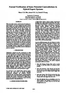
In order to illustrate the applicability and effectiveness of our methodology, we perform a case study on an advanced stateof-the-art Distributed DTM scheme, namely the Thermal-aware Agent-based Power Economy (TAPE) [7]. A. An Overview of TAPE The Thermal-aware Agent-based Power Economy (TAPE) [7] is an advanced distributed DTM approach for many-core systems organized in a grid structure. It employs the concept of a fully distributed agent-based system in order to deal with the complexity of thermal management in many-core systems. Each core is assigned its own agent which is able to negotiate with its immediate neighbors (i.e. adjacent cores, as depicted in Figure 2). Thermal management itself is performed by distributing power budgets which dictate task execution among the cores. Thus the agent negotiation consists of distributing this power budget based on the concept of supply-and-demand, taking the currently measured temperatures into account. Since each agent is only able to trade with its neighbors (east, west, north and south), multiple agent negotiations are required

to propagate power budget across the chip. At start-up, the available tasks are randomly mapped on the cores in the grid. Every core n keeps track of its f reen and usedn power units and new task assignment to a core results in increasing and decreasing its usedn and f reen power units, respectively, by a number that is determined by the requirements of the newly assigned task. Re-mapping of tasks is automatically invoked when either there are no free power units available in the node or the difference of temperatures in the neighboring nodes goes beyond certain threshold. The tasks are re-mapped to the nodes having the highest sellTn − buyTn values and thus the sellTn and buyTn values of a core govern its agent negotiations. Note: For better and clear understanding of the subsequent sections, system modeling and formal verification steps, terminology and parameters, we repeat the pseudo code of the TAPE in the appendix; see [7] for more details. Core

Agent

Agent Negotiation Agent properties: Scalable ÅÆ Agents act locally Situated ÅÆ Software entity in each core Social ÅÆMay negotiate with their neighbors Proactive ÅÆTriggered before threshold is reached Reactive ÅÆReacts to outside stimuli (i.e. from sensors) Light-weight ÅÆ Require small memory/computation footprint

Fig. 2: Overview of agent negotiation in TAPE

B. Modeling TAPE in PROMELA As discussed in Section III , the first step in our methodology (see Figure 1) is to construct the system model of TAPE DTM in PROMELA following the subsequent steps. Modeling Task Mapping and Re-Mapping: Task mapping and re-mapping is an essential component of TAPE. We developed structured macros, given in Algorithm 1, for these functionalities in PROMELA so that they can be called from the processes running in every core. The PROMELA keyword inline allows us to declare new functions, just like C. Both of these functions are called with two parameters, i.e., n, which identifies the node for task execution and the T T im, which represents the task time. The higher the value of T T im, the more power units it will consume and it is assumed that only 1 power unit is consumed for 1 time unit. As such the free power units are converted to used ones and the temperature is incremented by 4o C for each power unit (obtained from specific heat capacity of silica). In case of remapping, we have to find max(sellTn − buyTn ) according to [7] to find a suitable tile for mapping the task. The variable now is incremented in every execution of Algorithm 1 to keep track of the time. Variable Initialization Process: An initialization process, given in Algorithm 2, is used to initialize the data types for all the variables used in our model and perform the initial task mapping. The TAPE algorithm utilizes two normalizing factors, as and ab , to reflect temperature effects on the values of buyTn and sellTn and four weights ωu,b , ωu,s , ωf,b and ωf,s to reflect the effects of the variables usedn and f reen on the values of buybase and sellbase . All these variables are represented as real numbers in the TAPE algorithm of [7]. However, SPIN does not support real numbers and hence these variables must be discretized as explained in the previous section. The ranges

Algorithm 1 Structured Macros inline mapping(n,TTim) TTim:Task time { 1: nown = nown + T T im; 2: f reen = f reen − (T T im ∗ 1); 3: T mn = T mn + (T T im ∗ 4); 4: usedn = usedn + (T T im ∗ 1); } inline remapping(n,TTim) { 1: nown = nown + 1; 2: rmp = rmp + 1; 3: dn = sellTn − buyTn ; /*difference matrix */ 4: short mxm; 5: if 6: ::dn > mxm → mxm = dn ; /*finding max(sell-buy)*/ 7: ::else→skip; 8: fi; 9: if /*mapping*/ 10: ::mxm == dn → 11: nown = nown + T T im; 12: f reen = f reen − (1 ∗ T T im); 13: usedn = usedn + (1 ∗ T T im); 14: T mn = T mn + (4 ∗ T T im); 15: fi; }

of these variables can be found from the TAPE description [7]. For example, the values of normalizing factors, as and ab , must be bounded in the interval [0, 1]. Due to the inability to express real numbers, we use integers in the interval [1, 9] for assigning values to variables as and ab . In order to nullify the effect of this discretization on the overall behavior of the model, we have to divide the equations containing variables as and ab by 10 whenever they are used in the PROMELA model. Similarly, based on the behavior of the TAPE model, integers in the interval [0, 7] are used for the weight variables ωu,s , ωf,b and ωf,s and the interval [7, 14] for the weight variable ωu,b . Therefore, in order to retain the behavior of the TAPE model, we divide these variables by 7 whenever they are used (See e.g., Lines 11 and 12 of Algorithm 2). Algorithm 2 Initialization process P U : Power Units initialization process: init 1: select(wus : 1..6); 2: select(wfs : 1..6); 3: select(wub : 7..13); 4: select(wfb : 1..6); 5: select(as : 1..9); 6: select(ab : 1..9); 7: for all nodes n 8: f reen = P Utotal /(rows ∗ col); For even distribution of PU 9: usedn = 0; initially no used PU 10: T mn = T o; measured temperature is same as initial temperature

formally express any grid of arbitrary dimension. A node is modeled using two main processes, i.e., the receiver process, given in algorithm 3, that handles receiving values from the neighboring nodes and the agent process, given in algorithm 4, that is mainly responsible for processing the received values and then sharing them with the four neighbors of the node. The usage of the separate receiving process ensures reliable exchange of information as this way each node can receive information at any time irrespective of its main agent being busy or not. We have used both sending and receiving channels that are identified using the symbols ! and ? in the PROMELA model, respectively, for every node. Algorithm 3 Receiving Process n : identification of node proctype receiving(n,eastr,westr,northr,southr) 1: if receiving 2: ::eastr?buyTn , sellTn , time; → max(time, nown + 1) 3: ::westr?buyTn , sellTn , time; → max(time, nown + 1) 4: ::northr?buyTn , sellTn , time; → max(time, nown + 1) 5: ::southr?buyTn , sellTn , time; → max(time, nown + 1) 6: :: skip; 7: fi;

Discretization of the Temperature Variable: Finally, we also have to discretize the allowable increments and decrements for the temperature variable Tm , which is assigned the value of the initial temperature T0 = 30◦ C at start-up. For this purpose, we assume that the power units consumed for the execution time of a particular task amounts to 1mJ of energy. Thus, the worst-case temperature change that happens in one power unit consumption for the task can now be calculated to be approximately equal to 4◦ K using the relationship 1mJ/(CV ), where C represents the heat capacity equal to 1.547J·cm3 ·K−1 for Silica and V represents the volume of a core, which can be reasonably assumed to be equal to 1mm x1mm x150um. This discretization does not affect the verification objectives since we are only interested in the stability condition irrespective of the transient effects. Lamport Timestamps for Timing: We increment the value of nown whenever the node n gives a free power unit to one of its neighbors as a result of agent negotiation or whenever the values sellTn and buyTn are updated or whenever mapping, re-mapping, sending or receiving takes place.

initially

Iterative Model Construction and Verification Issues: It is worth mentioning that the above mentioned PROMELA model of TAPE was finalized after numerous runs through the proposed methodology, i.e., it had to go through deadlock checks and several stages of simplifications and optimizations.

Modeling of Many-Core System and TAPE’s Agent Process: The grid of cores (or tiles) of TAPE can be modeled as a two dimensional array of distributed nodes such that the TAPE algorithm runs on all these nodes concurrently. Based on the proposed methodology, we represented the behavior of these nodes using PROMELA processes and channels. We developed a generic node model so that it can be repeatedly used to

Issue-1: Deadlocks: We identified a deadlock in our first PROMELA model of TAPE, which occurred because a single channel was used to model both receiving and sending, which in turn lead to the possibility of missing the status update of a missing neighbor. To avoid this situation, we have used two different processes per node to model sending and receiving channels. Interestingly, this kind of a critical aspect, which prevents the system to achieve stability, was not mentioned or caught by the simulation-based analysis of TAPE that is reported in [7]. This point clearly indicates the usefulness of the proposed approach and using formal methods for the verification of distributed DTM schemes. Likewise, the above mentioned

11: sellbasen = (wus · usedn + wf s · f reen )/7 12: buybasen = (wub · usedn + wf b · f reen )/7 13: end for multiple task mapping is done randomly here instantiation of all agents and receiving processes are done here

These issues clearly indicate the shortcomings of simulation and are quite convincing to motivate the usage of formal methods for the verification of distributed DTM systems. Algorithm 4 Agent Process n : identification of node proctype agent(n,east,west,north,south) 1: sellTn = sellbasen + (as · (T mn − T o))/10; 2: buyTn = buybasen − (ab · (T mn − T o))/10; 3: if 4: :: (sellTn − buyTn ) − (sellTn [i] − buyTn [i]) > τ → 5: if 6: ::f reen > 0 → nown = nown + 1; f reen = f reen − 1; f reen [i] = f reen [i] + 1 7: ::else→ 8: nown = nown + 1; usedn = usedn − 1; f reen [i] = f reen [i] + 1; 9: if 10: ::tasktime > deadline → remapping(a, b, tasktime ); T mn = T mn − 4; 11: ::else→skip; 12: fi 13: fi 14: ::else → skip; 15: fi /*trading results in change of base buy/sell value*/ 16: if 17: ::(buyTn ! = lastbuyn ) || (sellTn ! = lastselln ) → 18: now = nown + 1; lastbuyn = buyTn ; lastselln = sellTn 19: east!buyTn , sellTn , nown ; 20: west!buyTn , sellTn , nown ; 21: north!buyTn , sellTn , nown ; 22: south!buyTn , sellTn , nown ; 23: :: skip; 24: fi;

V.

F ORMAL V ERIFICATION R ESULTS

A. Experimental Setup We use the version 6.1.0 of the SPIN model checker and version 1.0.3 of ispin along with the WINDOWS 7 Professional OS running on i7-2600 processor, 3.4 GHz(8 CPUs) with 16 GB memory. The verification is done for a 3x3 grid of nodes (cores) with all of them running the processes and channels described in the previous section. The complete model contains 18 processes and 350 lines of code. The SPIN utility BITSTATE is used for verification purposes since it uses 2808 Mb of space while allowing to work with up to 4.8 · 106 states.

Functional Verification Results: The most interesting functional characteristic to be verified in the context of TAPE is to ensure that the agent trading is always able to achieve a stable power budget distribution. For instance, it needs to be shown that no circular trading loops emerge where power budget is continuously traded preventing the system from stabilizing. Another possibility is that localized minima form which act as a barrier that prevents power budget from propagating. As a result, cores on one side of the barrier would no longer be able to obtain power budget even if it were available globally, and new tasks would be mapped to the other side of the barrier where power budget has accumulated. If such a scenario is possible, it would result in high temperatures and frequent remapping inside the region with the power budget not allowing the system to stabilize even though a global stable configuration would be possible. The non-occurrence of such instabilities can be ensured by verifying that “Eventually the sell-buy value between any two adjacent tiles would become very small". We have to verify 12 such properties so that all possible node pairs of a 3x3 grid are covered. For example, this property (p0001) can be expressed for nodes 00 and 01 as: [](((sell_T[0].vector[0]-buy_T[0].vector[0]) -(sell_T[0].vector[1]-buy_T[0].vector[1]) τn then 9: if any free power units are left then 10: decrement f reen 11: else 12: apply DVFS on n to get more free power units 13: decrement usedn 14: if the task does not meet the given deadline as DVFS is used then 15: (re-)mapping needs to be invoked 16: else 17: graceful performance degradation if allowed 18: end if 19: end if 20: increment f reei 21: end if 22: if buyTn = lastbuy or sellTn = lastsell then 23: send buyTn to all i ∈ N 24: send sellTn to all i ∈ N 25: lastbuy ← buyTn 26: lastsell ← sellTn 27: end if // This procedure will propagate until a stable state is reached. 28: end at 29: if received updated buy/sell values from any l ∈ Nn then 30: update buy[l], sell[l] 31: end if 32: if new task mapped to n requiring k power units then 33: f reen ← f reen − k 34: apply DVFS to PE on tile n 35: usedn ← usedn + k 36: end if 37: end for 38: end loop