Formalizing Cardinality-based Feature Models and their ... - CiteSeerX

Formalizing Cardinality-based Feature Models and their Specialization⋆ Krzysztof Czarnecki1 , Simon Helsen1 , and Ulrich Eisenecker2 2

1 University of Waterloo, Canada University of Applied Sciences Kaiserslautern, Zweibr¨ ucken, Germany

Abstract Feature modeling is an important approach to capture the commonalities and variabilities in system families and product lines. Cardinality-based feature modeling integrates a number of existing extensions of the original feature-modeling notation from Feature-Oriented Domain Analysis. Staged configuration is a process that allows the incremental configuration of cardinality-based feature models. It can be achieved by performing a step-wise specialization of the feature model. In this paper, we argue that cardinality-based feature models can be interpreted as a special class of context-free grammars. We make this precise by specifying a translation from a feature model into a context-free grammar. Consequently, we provide a semantic interpretation for cardinalitybased feature models by assigning an appropriate semantics to the language recognized by the corresponding grammar. Finally, we give an account on how feature model specialization can be formalized as transformations on the grammar equivalent of feature models.

Key words: Software product lines, system families, domain analysis, software configuration

1

Introduction

Feature modeling is a key approach to capture and manage the common and variable features in a system family or a product line.3 In the early stages of system family development, feature models provide the basis for scoping the system family by recording and assessing information such as which features are important to enter a new market or remain in an existing market, which features incur a technological risk, what is the projected development cost of each feature, etc. (DeBaud and Schmid, 1999). Later, feature models play a central role in the development of a system family architecture, which has to realize the variation points specified in the feature models (Czarnecki and Eisenecker, 2000; Bosch, 2000). In application engineering (also referred to as product development), which is the process of building individual systems based on the assets supplied by system family development, feature models can drive requirements elicitation and analysis. Knowing which features are available in the system family may help the customer to decide about the features his or her system should support. In particular, knowing which of the desired features are provided by the system family and which have to be customdeveloped helps to better estimate the time and cost needed for developing the system. A software pricing model could also be based on the additional information recorded in a feature model. Feature models also play a key role in generative software development (Czarnecki and Eisenecker, 2000; Greenfield and Short, 2004). Generative software development aims at automating application engineering based on system families: a system is generated from a specification written in one or more textual or graphical domain-specific languages (DSLs) (Weiss and Lai, 1999; Czarnecki and Eisenecker, 2000; Cleaveland, 2001; Batory, Johnson, MacDonald and von Heeder, 2002; Greenfield and Short, 2004). In this context, feature models are used to scope and develop DSLs (Czarnecki and Eisenecker, 2000; Deursen and Klint, 2002; Greenfield and Short, 2004), which may range from simple parameter lists or feature hierarchies to more sophisticated DSLs with graph-like structures. Feature modeling was proposed by Kang, Cohen, Hess, Nowak and Peterson (1990) as part of the Feature-Oriented Domain Analysis (FODA) method and since then it has been applied in a number of ⋆ 3

Preprint version of a paper to appear in Software Process Improvement and Practice 2005; 10(1) A system family is a set of systems built from a common set of assets such as a common architecture and a set of components, whereas a software product line additionally considers scoping and managing common product characteristics from the market perspective.

domains including telecom systems (Griss, Favaro and d’Alessandro, 1998; Lee, Kang and Lee, 2002), template libraries (Czarnecki and Eisenecker, 2000), network protocols (Barbeau and Bordeleau, 2002), and embedded systems (Czarnecki, Bednasch, Unger and Eisenecker, 2002). Pure::Variants (Beuche, 2004) is a commercial feature modeling tool, which is used by several automotive companies in Germany. Microsoft is integrating feature modeling into their software factories approach (Greenfield and Short, 2004). Based on this growing experience, a number of extensions and variants of the original FODA notation have been proposed (Griss et al., 1998; Czarnecki, 1998; Czarnecki and Eisenecker, 2000; Hein, Schlick and Vinga-Martins, 2000; van Gurp, Bosch and Svahnberg, 2001; Lee et al., 2002; Riebisch, B¨ollert, Streitferdt and Philippow, 2002; Czarnecki et al., 2002; Czarnecki, Helsen and Eisenecker, 2004b). 1.1

Contributions and Overview

This paper is based on our previous work on cardinality-based feature models (Czarnecki et al., 2004b). In that work, we introduced cardinality-based feature modeling as an integration and extension of existing approaches. We also introduced and motivated the notion of staged configuration. The present work adds a formal account of cardinality-based feature modeling and its specialization. The main contributions include a) a translation for cardinality-based feature models into context-free grammars, b) a semantic interpretation of feature models, and c) a set of informal grammar transformation rules which mimics feature model specialization steps. Our motivation for defining a formal semantics for cardinality-based feature models is threefold. First, this formal account aims at avoiding unnecessary misinterpretations and confusion about the meaning of the notation that may arise from an informal definition. For example, as reported by Bontemps, Heymans, Schobbens and Trigaux (2004), the “ambiguity problem” with respect to optional features in feature groups that was pointed out by Riebisch (2003) in the notation informally defined by Czarnecki and Eisenecker (2000) is actually a case of notational redundancy. This kind of confusion can be avoided by providing precise semantics. The need for formally defining a feature notation was also mentioned in the final report of the ECOOP Workshop on Modeling Variability for Object-Oriented Product Lines (Riebisch, Streitferdt and Pashov, 2004). Second, the presented semantics establishes a connection between cardinality-based feature modeling and the well-known formalism of grammars. Third, the process of formalization gave us a deeper understanding of various issues concerning the notation, which had impact on design decisions. For example, the addition of feature cardinalities represents a significant extension that has not been studied previously. In particular, it requires extending the notion of a configuration from a flat set of features to a structure that captures feature nesting. While the primary goal of our mapping of feature models to context-free grammars is to give our notation a precise meaning, a similar approach can also be used as an actual implementation mechanism. We discuss this possibility at the end of Section 4.2. The remainder of the paper is organized as follows: in Section 2, we describe cardinality-based feature modeling as it was proposed by Czarnecki et al. (2004b) and demonstrate it using a configurable editor as an example. Section 3 describes the notion of staged configuration as introduced by Czarnecki et al. (2004b). It is motivated and applied to the configurable editor example. The interpretation of feature models as context-free grammars is then detailed in Section 4. This includes the introduction of an abstract syntax model (Section 4.1), a translation into context-free grammars (Section 4.2), and a semantics for feature models (Section 4.3). Section 5 informally describes how feature model specialization steps have equivalent grammar transformation rules. Related work is discussed in Section 6 and Section 7 concludes.

2

Cardinality-Based Feature Modeling

In this section, we briefly describe cardinality-based feature modeling as it was proposed by Czarnecki et al. (2004b). For comparison with other approaches to feature modeling, we refer the interested reader to the original paper. A feature is a system property that is relevant to some stakeholder and is used to capture commonalities or discriminate among systems in a family (Czarnecki and Eisenecker, 2000). Note that while the original definition by Kang et al. (1990) has defined features as “user-visible” properties, we allow features with respect to any stakeholder, including customers, analysts, architects, developers, system administrators, etc. Consequently, a feature may denote any functional or non-functional characteristic at the 2

editorConfig

[0..*]

backup

autoSave

documentClass(String)

backupOnChange

backupExtension

associatedFileExtensions

commands

syntaxHighlighting

[0..*]

minutes(Int)

file.bak

file.bak.ext

ext(String)

file.ext.bak

syntaxDefinitionFile(String)

removeBlankLines Key:

f

f

Solitary feature with feature cardinality [1..1]

Solitary feature with feature cardinality [0..1]

[n..n’] Solitary feature with feature f cardinality [n..n’]

f1

spellCheck dosUnixConversion

Feature group with group cardinality (or if no cardinality f2 explicitly stated)

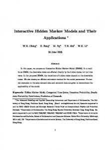
Figure 1. Text editor configuration example

requirements, architectural, component, platform, or any other level. Features are organized in feature diagrams. A feature diagram is a tree of features with the root representing a concept (e.g., a software system). Feature models are feature diagrams plus additional information such as feature descriptions, binding times, priorities, stakeholders, etc. As a practical example to demonstrate our cardinality-based language for feature modeling, consider the feature diagram of a configurable text editor in Figure 1. The root feature of our sample diagram is editorConfig. A root feature is only one of three different kinds of features. The other two are the grouped feature and the solitary feature. The former is a feature which occurs in a feature group, e.g., removeBlankLines. A solitary feature is a feature which is, by definition, not grouped in a feature group. Based on our experience in modeling embedded software and e-commerce systems, many features in a typical feature model are solitary, for example, the features backup and autoSave. The feature minutes is a subfeature of autoSave (i.e., minutes is a child of autoSave in the feature tree) and has an attribute for specifying the time period between automatic saves. In general, any feature can be given maximum one attribute by associating it with a type, which is Int in the case of minutes. A feature needs only at most one attribute since a collection of attributes can be easily modeled as a number of subfeatures, where each is associated with a desired type. If present, we indicate the associated type within parentheses after the feature name, e.g., myFeature (Int) . It is also possible to specify a value of the associated type immediately with the type, e.g., myFeature (5 : Int) . Every solitary feature is qualified by a feature cardinality.4 It specifies how often the entire subtree rooted in the solitary feature can be copied (with the roots of the replicated subtrees becoming siblings). For example, the features documentClass and ext have the feature cardinality [0..∗]. This means that an editor can be configured for zero or more document classes, each with zero or more associated file extensions. The feature cardinality of the remaining solitary features are implied by the filled or empty circle above the given feature as [1..1] or [0..1], respectively. For example, backup has the cardinality [1..1] (it is a mandatory feature), whereas the cardinality of autoSave is [0..1] (it is an optional feature). In general, a feature cardinality is defined as follows: Definition 1. A feature cardinality I is a sequence of intervals of the form [n1 ..n′1 ] . . . [nl ..n′l ], where we assume the following invariants: ∀ i ∈ {1, . . . , l − 1} : ni , n′i ∈ N nl ∈ N n′l ∈ N ∪ {∗} ∀n ∈ N : n < ∗ 0 ≤ n1 ∀ i ∈ {1, . . . , l} : ni ≤ n′i ∀ i ∈ {1, . . . , l − 1} : n′i < ni+1 4

More precisely, a feature cardinality is attached to the relationship between a solitary feature and its parent.

3

Throughout this paper N refers to the set of natural numbers including 0. An empty sequence of intervals is denoted by ε. An example of a valid specification of a feature cardinality with more than one interval is [0..2][6..6], which says that we can take a feature 0, 1, 2 or 6 times. Note that we allow the last interval in a feature cardinality to have as an upper bound the Kleene star ∗. Such an upper bound denotes the possibility to take a feature an unbounded number of times. For example, the feature cardinality [1..2][5..∗] requires that the associated feature is taken 1, 2, 5, or any number greater than 5 times. Semantically, the feature cardinality ε is equivalent to [0..0] and implies that the subfeature can never be chosen in a configuration. The available naming schemas for back-up files (such as file.bak or file.ext.bak) are modeled as a feature group. In general, a feature group expresses a choice over the grouped features in the group. This choice is restricted by the group cardinality hn– n′ i, which specifies that one has to select at least n and at most n′ distinct grouped features in the group. Definition 2. Group cardinality hn– n′ i of a group is an interval with n as lower bound and n′ as upper bound. Given that k > 0 is the number of grouped features in the group, we assume that the following invariant holds: 0 ≤ n ≤ n′ ≤ k. In our example, since no cardinality was specified for the group of naming schemas, the cardinality h1– 1i is assumed, i.e., the naming schemas form an exclusive-or group. Conversely, any combination of zero or more subfeatures of commands are allowed thanks to the group cardinality h0– 3i. At this point, we ought to mention that, theoretically, we could generalize the notion of group cardinality to a sequence of intervals, similarly as for feature cardinalities. However, we have found no practical applications of this usage and it would only clutter the presentation. Grouped features do not have feature cardinalities because they are not in the solitary subfeature relationship. This avoids redundant representations for groups and the need for group normalization which was necessary for the notation by Czarnecki (1998). For example, in that notation, an inclusiveor group—which has group cardinality h1– ki where k is the size of the group—can have both optional and mandatory subfeatures (corresponding to feature cardinalities [0..1] and [1..1], respectively). This would be equivalent to an inclusive-or group in which all the subfeatures were optional. Keeping feature cardinalities out of groups also avoids problems during specialization (see Section 3.2). For example, the duplication of a subfeature with a feature cardinality [n..n′ ], where n′ > 1, within a group could potentially increase its size beyond the upper bound of the group cardinality. Observe that, even without the redundant representations for groups, there is still more than one way to express the same situation in our notation. For example, the feature group with group cardinality h0– 3i under the feature commands in Figure 1 can also be modeled as in Figure 2.

commands

[0..1] removeBlankLines

[0..1] spellCheck

[0..1] dosUnixConversion

Figure 2. Alternative representation for commands

We keep the representation in Figure 2 distinct from the representation in Figure 1 and leave it up to a tool implementer to decide how to deal with these multiple representations. For instance, it might be useful to provide a conversion function for such diagrams. Alternatively, one could decide on one type as the preferred form which is shown by default.

3

Staged Configuration

A feature model describes the configuration choices within a system family. An application engineer may specify a member of a system family by selecting the desired features from the feature model within the 4

variability constraints defined by the model (e.g., the choice of exactly one feature from a set of alternative features). The process of specifying a family member may also be performed in stages, where each stage eliminates some configuration choices. We refer to this process as staged configuration. Staged configuration can be achieved through subsequent specialization of a feature model in each stage. In this approach, each stage takes a feature model and yields a specialized feature model, where the set of systems described by the specialized model is a subset of the systems described by the feature model to be specialized.5 The need for staged configuration arises in at least three contexts: Software supply chains In software supply chains (Greenfield and Short, 2004), a supplier can create families of software components, platforms, and/or services dedicated for different system integrators based on one common system family, which covers all the variability needed by the individual families. In general, a similar relationship can exist between tier-n and tier-n+1 suppliers of the system integrator. This creates the need for multi-stage configuration, where each supplier and system integrator is able to eliminate certain variabilities in order to create specialized system families and to compose such specialized families. We provide an example involving embedded software in the automotive industry elsewhere (Czarnecki et al., 2004b). Optimization Staged configuration offers an opportunity to perform optimizations based on partial evaluation (Jones, Gomard and Sestoft, 1993). When certain configuration information becomes available at some stage and it remains unchanged thereafter, the software can be optimized with respect to this information. For example, configuration information available at compile-time can be used to eliminate unused code from a component and to perform additional compile-time optimizations. Similarly, the component could be further specialized based on configuration information available at deployment time. Optimizations are especially interesting for embedded software and software that needs to be distributed over the net. Note that optimization stages may coincide with the configuration stages within a supply chain, but this is not always the case. Many suppliers decide to deploy runtime keys to enable or disable certain product features without physically eliminating the unused code.6 Policy standards Infrastructure policies may be defined at different levels of an organization with the requirement of hierarchical compliance. For example, security policy choices provided by the computing infrastructure of an enterprise can be specialized at the enterprise level, then further specialized at the level of each department, and finally at the level of individual computers. A concrete example of specializing security policies can be found elsewhere (Czarnecki et al., 2004b). Configuration stages can be defined in terms of three different dimensions:7 Time A configuration stage may be defined in terms of the different phases in a product lifecycle (e.g., development, roll-out, deployment, normal operation, maintenance, etc.). These times are, of course, product-specific. They will have to be mapped to the different binding times offered by the utilized technologies (e.g., compile-time, preprocessing time, template-instantiation time, load time, runtime, etc.). Targets A target system or subsystem for which a given software needs to be configured may also define possible configuration stages. For example, a given component may be deployed several times within a given software system. In this case, the component could first be specialized to eliminate functionality not needed within the system and then be further configured for each deployment context within that system. Roles In staged configuration scenarios, eliminating different variabilities may be the responsibility of different parties, which can be assigned different roles. For example, a central security group may 5

6

7

In some application contexts, staged configuration requires independently defined feature models for each stage. The latter is achieved by multi-level configuration. The notion of multi-level configuration is described elsewhere (Czarnecki, Helsen and Eisenecker, 2004a). The choice of employing runtime techniques for static configuration may sometimes be dictated by the limitations of the implementation technology being used. However, there may be more profound reasons, such as logistics requiring packaging all variants into a single distribution (Czarnecki et al., 2002, pp. 168-169). The notion of binding time in feature modeling with respect to implementation technologies was introduced by Kang et al. (1990). The generalized set of binding dimensions (i.e., time, target, and roles) corresponds to modeling the “when, where, and by whom features are bound” as proposed by Czarnecki (1998, p. 98).

5

be responsible for defining enterprise-wide security polices, while the configuration of the individual computers may be done by the departmental system administrators. Similarly, multiple configuration roles will be typically required in a supply-chain scenario. 3.1

Configuration vs. Specialization

So far, we have loosely defined the terms feature model specialization and feature model configuration. At this point, it is important to make these notions more precise. A configuration consists of the features that were selected according to the group and feature cardinalities defined by the feature diagram. The relationship between a feature diagram and a configuration is comparable to the one between a class and its instance in object-oriented programming. The process of deriving a configuration from a feature diagram is also referred to as the configuration process. The specialization process is a transformation process that takes a feature diagram and yields another feature diagram, such that the set of the configurations denoted by the latter diagram is a subset of the configurations denoted by the former diagram. We also say that the latter diagram is a specialization of the former one. A fully specialized feature diagram denotes only one configuration. In general, we can have the following two extremes when performing configuration:8 a) deriving a configuration from a feature diagram directly and b) specializing a feature diagram down to a fully specialized feature diagram and then deriving the configuration (which is trivial). Observe that we might not always be interested in one specific configuration. For example, a feature diagram that still contains unresolved variability could be used as an input to a generator. This is useful when generating a specialized version of a framework (which still contains variability) or when generating an application that should support the remaining variability at runtime. 3.2

Specialization Steps

Specialization of a feature diagram can be achieved by applying specialization steps to it. There are six categories of specialization steps: (1) refining a feature cardinality, (2) refining a group cardinality, (3) removing a subfeature from a group, (4) selecting a subfeature from a group, (5) assigning a value to an attribute which only has been given a type, and (6) cloning a solitary subfeature. We discuss each of these possibilities in more detail. Refining feature cardinalities A feature cardinality is a sequence of intervals representing a (possibly infinite) set of distinct natural numbers. Each natural number in the cardinality stands for an accepted number of occurrences for the solitary subfeature. Refining a feature cardinality means to eliminate elements from the subset of natural numbers denoted by the cardinality. This can be achieved as follows: 1. remove an interval from the sequence; or 2. if an interval is of the form [ni ..n′i ] where ni < n′i , (a) reduce the interval by increasing ni or decreasing n′i as long as ni ≤ n′i holds for the reduced interval. If n′i = ∗ in the original interval, then it is possible to replace ∗ with a number m such that ni ≤ m; or (b) split the interval in such a way that the new sequence still obeys the feature cardinality invariant and then reduce the split intervals according to rule 2a. A special case of refining a feature cardinality is to refine it to [0..0] or ε. In either case, it means we have removed the entire subfeature and its descendants. We leave it up to a tool implementation to decide whether to visually remove features with feature cardinality [0..0] or ε. Refining group cardinalities A group cardinality hn1 – n2 i is an interval indicating a minimum and maximum number of distinct subfeatures to be chosen from the feature group. Its form is a simplification of a feature cardinality and can only be refined by reducing the interval, i.e., by increasing n1 or by decreasing n2 as long as n1 ≤ n2 . Currently, we do not allow to split an interval, because we have no representation for such a cardinality. Of course, such an operation should be incorporated whenever we allow sequences of intervals for group cardinalities. 8

We usually drop the term “process” from “configuration process” and “specialization process” when the intended meaning is clear from the context.

6

Removing a subfeature from a group A feature group of size k with group cardinality hn1 – n2 i combines a set of k subfeatures and indicates a choice of at least n1 and at most n2 distinct subfeatures. A specialization step can alter a feature group by removing one of the subfeatures (including the entire subtree rooted in this subfeature), provided that n1 < k. The new feature group will have size k − 1 and its new group cardinality will be hn1 – min(n2 , k − 1)i, where min(n, n′ ) takes the minimum of the two natural numbers n and n′ . Figure 3 shows a sample specialization sequence where each step removes one subfeature from a group. Each arrow denotes an application of one specialization step. It is not possible to remove subfeatures from a feature group once n1 = k. In that case, all subfeatures have to be taken and all variability is eliminated.

f

f

f

f

1

f

f

2

3

f

4





f

f

1

f

2

f

3

f

1

2

Figure 3. Example of specialization by removing group members

Selecting a subfeature from a group A specialization step can alter a feature group of size k with group cardinality hn1 – n2 i by selecting one of the subfeatures, provided that n2 > 0. The new feature group will have size k − 1 and its new group cardinality will be h(max(0, n1 − 1))– (n2 − 1)i, where max(n, n′ ) takes the maximum of the two whole numbers n and n′ . Figure 4 shows a sample specialization sequence where each step selects one subfeature from a group. It is not possible to select subfeatures from a feature group once n2 = 0. In that case, the group has been essentially removed.

f

f



f

1

f



f

2

f

3

f

4

f



f

1

2

f

3

f

4

f

1

f

2

f

3

f

4

Figure 4. Example of specialization by selecting group members

Assigning an attribute value An obvious specialization step which assigns a value to an uninitialized attribute. The value has to be of the type of the attribute. Cloning a solitary subfeature This operation makes it possible to clone a solitary subfeature and its entire subtree, provided the feature cardinality allows it. Moreover, the cloned feature may be given an arbitrary, but fixed, feature cardinality by the user, as long as it is allowed by the original feature cardinality of the solitary subfeature. Unlike the other specialization operations, it is possible that cloning only changes the diagram without removing variability. However, the new diagram will generally be more amenable to specialization, so we consider it a specialization step nonetheless. We explain this process with an example in Figure 5. The feature cardinality [2..2][4..∗] of the original subfeature f0 indicates that f0 must occur at least 2 times or more than 3 times in a configuration. In 7

f

f

[3..3]

[2..2][4..*]

f

[1..*]

f0

0

f0

Figure 5. Example of specialization by cloning

the specialized diagram above, we have cloned f0 (to the left) and assigned it a new feature cardinality [3..3]. The original feature f0 (to the right) has a new cardinality that guarantees that the new diagram does not allow configurations which were previously forbidden. In the example, because we have chosen to give the left f0 the fixed feature cardinality [3..3], the feature cardinality of the right-most f0 has to be [1..∗]. Specialization has occurred since the new diagram does not allow a user to only select f0 two times.

f

f

[2..*]

f

[0..*]

[2..2]

f1

1

f1

Figure 6. Example of cloning with no specialization

Consider another example in Figure 6. In this example, no actual specialization took place. The cloned feature f1 to the left has been given the fixed cardinality [2..2]. However, because the original feature cardinality was [2..∗], the right-most f1 now has cardinality [0..∗].

f

f

[m..m]

I

f’

f’

L(m,I) f’

Figure 7. General form of the cloning step

More generally, suppose I = [n1 ..n′1 ] . . . [nl ..n′l ] and 0 < m. Provided we have (n′l = ∗) ∨ (m ≤ n′l < ∗), it is possible to clone the solitary subfeature f ′ of f with feature cardinality I as shown in Figure 7. This is the general form of the cloning step. Given that we always have ∗ − n = ∗ for any n ∈ N, we can define the function L (m, I) as follows: Definition 3. L (m, ε) = ε  if (m ≤ n) : [(n − m)..(n′ − m)]L (m, I) ′ L (m, [n..n ]I) = if (n < m) ∧ (m ≤ n′ ) : [0..(n′ − m)]L (m, I)  if n′ < m : L (m, I)

Note that the function definition uses juxtaposition to express construction and destruction of a sequence of objects. For example, I = [n..n′ ]I′ implies that [n..n′ ] is the head of the sequence I and I′ is its tail. 8

editorConfig

backup

documentClass(¨Java¨ : String)

documentClass(¨binary¨ : String)

syntaxHighlighting autoSave

backupOnChange

backupExtension

associatedFileExtensions

commands

associatedFileExtensions syntaxDefinitionFile(¨java.syn¨ : String)

[0..*]

minutes(Int)

file.bak

file.bak.ext

file.ext.bak

[0..*]

ext(String)

ext(¨dll¨ : String)

ext(¨exe¨ : String)

ext(String)

commands

ext(¨java¨ : String) removeBlankLines

dosUnixConversion

Figure 8. Sample specialization of the editor configuration

The reader may wonder why we only allow the cloned feature to be given a fixed feature cardinality. This is because it is not always possible to construct a correct feature diagram by cloning a feature and giving it an arbitrary interval or sequence of intervals without some more expressive form of additional constraints. However, there are a few useful special cases for this situation, which we do not consider in this paper and leave for future work. 3.3

Editor Configuration Example Revisited

Coming back to our editor configuration example in Section 2, assume that the developer of the editor decides to create specialized editors for different markets. For example, a specialization for programmers might support editing Java files and viewing binary files (see Figure 8). The specialization is achieved by a combination of steps from Section 3.2: refining the feature cardinalities for autoSave and backupOnChange to [1..1]; cloning documentClass once and refining the feature cardinality of the original documentClass to [1..1]; assigning names to both documentClasses; cloning ext and assigning names to each of the clones; deleting selected features from the groups under commands; and refining the group cardinality for the commands of the Java document class to h2– 2i. The specialized feature diagram could be used as the input to a generator or as a start-up configuration file. The remaining variability could be exposed to the end-user through a properties dialog box in the generated editor.

4

Feature Models as Context-Free Grammars

Our approach to formalize cardinality-based feature models is based on a translation of feature diagrams into context-free grammars. A formal semantics for a feature model is then obtained by an appropriate interpretation of the sentences recognized by the corresponding grammar. Before we can translate cardinality-based feature models into grammars, we need to define an abstract syntax that will simplify the design of the translation algorithm compared to working directly on the concrete syntax. The abstract syntax will be defined as a meta model plus a notation to describe concrete instances of the meta model. 4.1

Abstract Syntax for Feature Diagrams

Usually, an abstract-syntax model is engineered to accommodate the expressiveness of the meta modeling language. For example, if the meta model is expressed as a UML model, sound object-oriented design principles are used. In our case, however, we want the abstract syntax to be easily manipulable by a translation algorithm. This requires more orthogonality of the different language elements and may not necessarily lead to the most intuitive meta model. Still, for improved readability, we formalize the abstract syntax model with a UML class diagram because this standardized notation is readily understandable. Figure 9 contains the meta model for the 9

is subfeature of

*

children

Subfeature Relationship

Node name

featureCardinality 0..1

parent

Grouping Node

Feature Node

groupCardinality 1..* children

0..1

parent

feature group

Figure 9. Abstract syntax meta model for cardinality-based feature models

proposed abstract syntax of our cardinality-based feature notation.9 An abstract syntax feature diagram consists of nodes which can be either feature nodes or grouping nodes. Each node has a name which refers to the actual feature name. Note that we differentiate between a feature name and a feature node. As is the case in the concrete syntax, feature names do not have to be unique. However, each feature node is a unique object. A feature node may have a set of zero or more subnodes via the subfeature relationship, which in itself has a feature cardinality. Solitary subfeatures from the concrete syntax are thus represented in the abstract syntax as a node with an is-subfeature-of link. A grouping node, on the other hand, has at least one or more subfeature nodes in its feature group. Observe that a grouping node cannot have an empty feature group because if a node has no children, it must be a feature node. In addition to the diagram constraints of Figure 9, we have three implicit constraints: a) a grouping node always has an associated subfeature link; in other words, a diagram cannot have a grouping node as its root; b) the feature cardinality of the subfeature link associated with a grouping node is always [1..1]; c) an abstract syntax feature diagram is always a proper tree, i.e., a node cannot appear as one of its descendants. Although attributes are a useful and important aspect of the feature notation presented in this paper, we do not consider features with attributes in the formalization of feature models. This extension only clutters the presentation. In Section 4.2 we informally discuss how attributes can be added to the formalization. Let us now consider a concise notation for the abstract syntax. A feature node and its subfeatures with associated feature cardinality have the following form:   I1 f1   f  ...   In fn In this case, f is a feature node, whereas f1 , . . . , fn are its subnodes, which can be either features or grouping nodes. Note that in this notation, we mix feature names and feature nodes because we can uniquely determine which node we are talking about by observing its position in the tree. The feature cardinality Ii of a subfeature relationship precedes the feature node it is qualifying. A grouping node of size k (i.e., with k subfeatures) is presented as follows:  f1   . ′  . g hn– n i   .  fk

The interval hn– n′ i is the group cardinality. The concrete syntax can now be easily mapped onto the abstract syntax as explained in Figure 10. It is relatively straightforward to check that this mapping obeys the implicit constraints on the abstract syntax mentioned above. 9

Contrast this with the meta model proposed by Czarnecki et al. (2004b).

10

We finish this section with a sample feature diagram and its abstract syntax representation in Figure 11. We will use this feature diagram in the remainder of the paper to explain the formalization of cardinality-based feature models.

f

f|

f

? ? .. ?. ? ′ f? ?If | ?. ? ..

I f’

? ?. ? .. ? 8 ? f1 | ? > > ? >. ′ > ? > .. f ? [1..1] g hn– n i > > > ? : ? fk | ? ? .. ?.

f

f

f

1

k

Figure 10. Mapping from concrete to abstract syntax

f

? ? [1..2][4..∗] f1 | 8 ? ? f2 | > ? [1..1] g h1– 1i > : ? f3 | ? ? ? ? [0..∗] f5 | ? ? 8 f? ? f6 | > ? ? > > ? [0..2] f4 ? > f7 | > ? ? [1..1] g h2– 3i > > ? ? > > ? ? : f8 | ? ? f3 |

[1..2][4..*]

f1

[0..2]

f2

f3

f4

[0..*]

f5

f

6

f

7

f

8

f

3

Figure 11. A sample feature diagram and its abstract syntax representation

4.2

A Translation into Context-Free Grammars

As mentioned earlier, our approach to the formalization of a feature diagram is to translate it into a context-free grammar. Feature diagrams, as they are presented in this paper, can actually be modeled as 11

regular grammars 10 and do not require the additional expressiveness of context-free grammars. However, because regular grammars are rather awkward to read, we will present a translation into a more convenient context-free grammar. An informal description We first explain the translation into context-free grammars by means of the example in Figure 11. The notation for context-free grammars is standard, but for improved readability, we print non-terminals in italic and underline terminals. The translation consists of two parts: translating feature nodes and translating grouping nodes. First, let us look at how to deal with feature nodes, for example the root feature node f of the example. It has three subfeature links with associated nodes f1 , g, and f4 . For the root feature f , we generate the following production: Ff 1 → ( f , Nf 1 f11 ∪ Nf 1 g 2 ∪ Nf 1 f43 ) . Although feature names are generally not unique, an actual feature node occurring in a diagram is. Hence, we use an encoding that guarantees that the non-terminal corresponding to a particular node in the diagram is unique. It works as follows: Each abstract syntax node is represented by a non-terminal Fid . The subscript id is a sequence of node names describing the path of the root node all the way down to the current node. Moreover, each node name itself is superscripted with an index that distinguishes it from all its siblings.11 In theory, it is sufficient to only use the superscripts without the node names to form a unique identity for the non-terminal. However, it is easier to read the productions when we add the node names to the identity. We use the same method for other non-terminals such as N and G that describe different aspects of the same diagram node. In the above production, we see the non-terminals Nf 1 f11 , Nf 1 g 2 , and Nf 1 f43 . They encode the possible number of occurrences according to the feature cardinality of the respective feature. For example, let us investigate what happens with the case for Nf 1 f11 . It requires four productions: Nf 1 f11 → { Nf11 f 1 }

Nf 1 f11 → { Nf21 f 1 }

1

Nf 1 f11 → {

Nf41 f 1 1

1

}

Nf 1 f11 → {

Nf51∗f 1 1

}

Each right-hand side is a non-terminal, enclosed in curly brackets to represent the different numbers that the feature cardinality represents. Because the final interval has a Kleene star, it is possible to go to the non-terminal Nf51∗f 1 . Each of these numbered non-terminals is then elaborated in a production 1 that goes to the non-terminal representation of the subnode. For node f1 , this implies the following productions: Nf11 f 1 → Ff 1 f11 Nf21 f 1 → Ff 1 f11 , Ff 1 f11 1

Nf41 f 1 1

1

→ Ff 1 f11 , Ff 1 f11 , Ff 1 f11 , Ff 1 f11

Nf51∗f 1 → Ff 1 f11 , Nf41 f 1 1

Nf51∗f 1 → Ff 1 f11 , Nf51∗f 1 1

1

1

The first three productions are obvious. The last two productions take care of the interval [5..∗]. The Kleene star requires a recursive production to represent an unbounded number of f1 , but always ends by taking at least 5 of those features. Note that we insert a comma terminal symbol in between occurrences of Ff 1 f11 . That is to make sure we can interpret the result sentence appropriately. The interpretation of resulting sentences is discussed below. The cases for Nf 1 g 2 and Nf 1 f43 are analogous. If the feature cardinality allows for 0 occurrences, as is the case for Nf 1 f43 , we have to include a production Nf01 f 3 → ǫ. Finally, we have to consider the case 4 where a feature has no subfeature links at all. This is the case for feature f1 , where we have the production Ff 1 f11 → ( f1 , ∅ ) . 10

11

Regular grammars require that the right-hand side of a production can only have one terminal possibly followed by a non-terminal. In many of the examples in this paper, we use subscripts of f to identify different feature names, e.g., f1 . However, these subscripts are part of the actual feature name and should not be confused with the indices that identify siblings.

12

Now, let us look at the translation of a grouping node. From the example diagram in Figure 11, we take the grouping node g of the feature f4 , which has group cardinality h2– 3i and four subfeatures f6 , f7 , f8 , and f3 . This means that we have to generate productions that accept all combinations of minimum 2 and maximum 3 distinct subfeatures. As with feature cardinalities, we directly encode all possible numbers in the interval of the group cardinality with extra non-terminals. However, unlike feature nodes, we do not produce a terminal for the grouping node because it is only an artifact of the abstract syntax: Ff 1 f43 g 2 → Gf21 f 3 g 2

Ff 1 f43 g 2 → Gf31 f 3 g 2

4

4

In the next step, we have to produce all the combinations for each number in the interval. A possible choice of subnodes is comma-separated. For example, for Gf21 f 3 g 2 , we have the following productions: 4

Gf21 f 3 g 2 → Ff 1 f43 g 2 f61 , Ff 1 f43 g 2 f72

Gf21 f 3 g 2 → Ff 1 f43 g 2 f61 , Ff 1 f43 g 2 f83

Gf21 f 3 g 2 4

Gf21 f 3 g 2 4

4

4

→ Ff 1 f43 g 2 f61 , Ff 1 f 3 g 2 f 4 4

3

Gf21 f 3 g 2 → Ff 1 f43 g 2 f83 , Ff 1 f 3 g 2 f 4

Gf21 f 3 g 2 → Ff 1 f43 g 2 f72 , Ff 1 f 3 g 2 f 4 4

4

→ Ff 1 f43 g 2 f72 , Ff 1 f43 g 2 f83

3

4

4

3

The productions for Gf31 f 3 g 2 are analogous. The context-free grammar is completed by identifying 4 the start symbol, which is the non-terminal representing the root feature node. In our example, this is Ff 1 . The complete translation of the example in Figure 11 can be found in Appendix A.

A translation algorithm We now
provide a complete algorithm, written in pseudo-code. It consists of a large recursive function T . . . which takes as one of its arguments an abstract syntax node and produces a set of grammar productions. The notation used in the pseudo-code is largely self-explaining. We use the symbol α for a sequence of grammar symbols, which may contain both terminals and non-terminals. As previously noted, juxtaposition expresses construction and destruction of a sequence of objects. For example, I = [n..n′ ]I′ implies that [n..n′ ] is the head of the sequence I and I′ is its tail. The symbol ξ stands for a sequence of feature names.
We use pattern matching on the type of the parameter of the function T . . . . According to the meta model in Figure 9, the parameter is a node object that can be either a feature node
or a grouping node. The function T dispatches accordingly. The translation starts with T ε, 1, f . . . , where f is the root feature of the diagram. First, we specify the case for a feature node: Definition 4.    if n = 0 : { Fξ′ → ( f , ∅ ) }         if n > 0 : { Fξ′ → ( f , Nξ′ f11 ∪ . . . ∪ Nξ′ fnn ) } ∪  I1 f1 . . .          if Ii = ε : { Nξ′ fii → ∅ } T  ξ, m, f  ... =   n  [   In fn . . .    if Ii 6= ε : N ( Nξ′ f i , Ii , Fξ′ f i )      i i  
 i=1  ′ ∪ T ξ , i, fi . . . where ξ ′ = ξf m

It needs a function which generates productions for each number in the feature cardinality. 13

Definition 5.  if I = ε : ε        I = [n1 ..n2 ]I′ ∧    if : { N → { N n1 } } ∪  n1 < n2 < ∗    N ( N , [(n1 + 1)..n2 ]I′ , F ) ∪     N ′ ( N n1 , n1 , F )         I = [n..n]I′ ∧   if : { N → { N n } } ∪ N ( N , I′ , F ) ∪   n 0 : { N → N ′′ (n, F )}

Definition 7. N (n, F ) = ′′

(

if n = 1 : F if n > 1 : F , N ′′ (n − 1, F )

Now, we consider the case for a grouping node: Definition 8.  if n′ = 0 : { Fξ′ → ǫ}        if 0 < n = n′ : { Fξ′ → Gξn′ } ∪     G( Gξn′ , n, ξ ′ , fk . . . f1 ) ∪    k  [ 
  (T ξ ′ , i, fi . . . )  

  f1 . . .   .   i=1  . T  ξ, m, f hn– n′ i  =    . ′   if n < n : { Fξ′ → Gξn′ } ∪ fk . . .     G(  Gξn′ , n, ξ ′ , fk . . . f1 ) ∪       f1 . . .      .      .. T  ξ, m, f hn′′ – n′ i          f ... 

k

′

where ξ = ξf

m

′′

and n = n + 1

It requires two functions G and G ′ , which are very similar. Together, they generate all possible combinations of n subfeatures for the grouping node. We need two functions because we have to deal separately with the first selected feature and any possibly remaining features because of the comma separation. Note that for the case n = k, we have to take all subfeatures. In case we have n < k, we can either select the subfeature or not. 14

Definition 9.  if n = 0 : { G      if 0 < n < k : G( G, n, ξ, fk . . . f1 ) =      if 0 < n = k :

→ ǫ} G ′ ( G, Fξfkk , n − 1, ξ, fk−1 . . . f1 ) ∪ G( G, n, ξ, fk−1 . . . f1 ) G ′ ( G, Fξfkk , n − 1, ξ, fk−1 . . . f1 )

Definition 10.

 if n = 0 : { G      if 0 < n < k : G ′ ( G, α, n, ξ, fk . . . f1 ) =      if 0 < n = k :

→ α} G ′ ( G, α′ , n − 1, ξ, fk−1 . . . f1 ) ∪ G ′ ( G, α, n, ξ, fk−1 . . . f1 ) G ′ ( G, α′ , n − 1, ξ, fk−1 . . . f1 )

where α′ = Fξfkk , α

A Note on Space Complexity The presented translation into context-free grammars satisfies the goal of this paper to provide precise semantics for cardinality-based feature modeling. However, the translation is not appropriate to be used as an implementation approach for feature modeling as is. This is because the translation algorithm creates a separate production for each valid combination of features from a group, and, consequently, the number of grammar productions created for a feature group may grow exponentially. For example, for an inclusive-or group with k features, 2k − 1 productions will be generated. In general, an implementation of feature modeling via grammars would use a two-phase process to validate a feature model. First, a feature model would be validated with respect to a grammar. Second, if the model passed the first test, it would be checked with respect to global constraints, i.e., constraints between features in different parts of a feature diagram, and those local constraints that were not captured by the grammar. For example, this approach is used by Cechticky, Pasetti, Rohlik and Schaufelberger (2004), in which a feature model is translated into XML Schema plus XSLT rules encoding global constraints. An XML document representing a configuration is first checked by a validating XML parser. After successfully passing the first test, the XSLT rules are applied.12 The combinatorial explosion can be easily avoided in a practical implementation. This can be achieved by converting each group with group cardinality hn– n′ i, where n′ > 1, into a set of optional solitary features. The additional semantics of the original group (i.e., that the number of selected features lies within the group cardinality interval) would be expressed by constraints to be checked in the second phase. Our translation does not use this approach in order to have a uniform grammar-based definition of semantics for the entire notation. 4.3

Semantics of Feature Models

In general, the semantics of a feature model can be defined by the set of all possible configurations captured by the feature model. A configuration itself is denoted by a structured set of features, which are chosen according to the informal rules of interpretation of feature diagrams. Although this description is sufficient in practice, it is helpful to provide a more formal semantics to improve the understanding of some of the intricacies of feature modeling. For example, a formal semantics allows us to define exactly what it means when two apparently different feature models are equivalent, i.e., when they denote the same set of configurations. Consider the context-free grammar generated from a cardinality-based feature model. We define the semantics of a feature model as an interpretation of the sentences from the language recognized by the grammar. 12

It is interesting to note that the XML approach by Cechticky et al. (2004) was applied on a project in the context of configuring embedded systems, even though the approach also used a combinatorial translation for groups. However, it may be that the project had no groups causing a combinatorial explosion (such as inclusive-or groups) or each group had only a few members.

15

Each individual sentence of the recognized language corresponds to exactly one configuration. For example, the following string is recognized by the grammar in Appendix A and thus, represents a valid configuration of the feature diagram in Figure 11: (f, {(f1 , ∅), (f1 , ∅)} ∪ {(f3 , ∅)} ∪ {(f4 , {(f5 , ∅)} ∪ {(f6 , ∅), (f3 , ∅)})}) Although the string is nothing more than a sequence of terminals, we can assign it a semantic interpretation as follows: “each pair is an element from the relation between features (identified by their feature names) and their multiset of subfeatures”. The semantics of the entire feature model is now defined as the set of all such configurations. There are a few observations to make at this point: – The sentences representing configurations still contain the tree structure of the feature diagram via the nested pairs of features and their subfeatures. This is important because a configuration not only represents what features are selected but also how they fit in the hierarchy. This nesting information is required because of cloning. In contrast, feature notations that do not support cloning, such as the FODA notation, can represent configurations as flat sets of features. In order to understand why we want to keep the nesting information in a configuration in the presence of cloning, consider our example in Figure 11. Suppose that we represented configurations as flat sets and a particular configuration had two f4 and two f5 . Without nesting information, we would not know whether both f5 in the configuration were children of just one f4 or each f4 had one f5 as its child. – The second element of a pair is a multiset, not a set. This implies that each occurrence of the same feature name is semantically relevant for a configuration. Moreover, we cannot use sequences to represent subfeatures, because the order in which features are chosen is not relevant for the result configuration. – The semantics of feature diagrams via context-free grammars is layered: first, we interpret a feature model as a language that the corresponding grammar recognizes. Second, we interpret the recognized language in a standard mathematical way to obtain a denotation for the feature model. – It is relatively easy to add attribute types to the generated grammar. For a feature f with an attribute of type t, we want to be able to construct a configuration triple consisting of the feature f , a value v of the type t, and a multiset of possible subfeatures. In the production of the feature f , we have a non-terminal T t at the position for the value. The non-terminal represents the type t at the grammar level. This is achieved by a set of productions with left-hand side T t , encoding all possible values in t. The semantics of the feature diagram will now include all possible configurations with a particular value of the type t. If a feature diagram has already assigned a value v to the attribute, we can simply adapt the productions for T t in such a way that they only recognize v. In this case, the adapted productions for T t actually stand for the singleton type {v}.

5

Feature Model Specialization and Context-Free Grammars

In Section 3.2, we discussed the possible specialization steps to achieve staged configuration of feature models. Specialization of a feature model can also be interpreted on the level of its grammar equivalent. 5.1

Specialization as a Grammar Transformation

In this section, we give an informal discussion on how to achieve each individual specialization step of Section 3.2 by grammar transformations, where we omit the initialization of attributes. We do not provide a formal algorithm because it would unnecessarily clutter the exposition. Instead, we explain the different specialization operations by means of the example feature diagram in Figure 11. Refining feature cardinalities Consider the feature cardinality [1..2][4..∗] of the feature node for f1 . This cardinality is represented by the production rules with left-hand side Nf 1 f11 . In Section 3.2, we gave several possibilities to refine a feature cardinality, including the removal of an interval, reducing an interval and splitting it. On the level of the grammar, this amounts to removing the productions that stand for any of the numbers 1, 2, and 4 from the cardinality. In other words, delete the 16

production Nf 1 f11 → { Nfi1 f 1 } , where i ∈ {1, 2, 4}. The reduction of the interval [4..∗] to [4..4] simply 1 requires the removal of Nf 1 f11 → { Nf51∗f 1 } . 1 Observe that the removal of these kind of productions leaves several more productions in the grammar unreachable, i.e., they are never used whenever we try to accept a sentence starting with the start symbol. In the remainder of this section, we will assume that unreachable productions are automatically garbage collected. The nature of the grammar has excluded one category of refinement so far: the reduction or splitting of [4..∗] into two intervals [4..m] and [m..∗], where m > 4. That is because the encoding of the Kleene star at the grammar level uses recursion. In order to achieve a refinement of [4..∗] involving a number m > 4, we have to unroll the productions that encode the Kleene star. In the example, suppose we want to split [4..∗] into [4..6][7..∗], we have to replace the productions Nf 1 f11 → { Nf51∗f 1 } , Nf51∗f 1 → Ff 1 f11 , Nf41 f 1 , and Nf51∗f 1 → Ff 1 f11 , Nf51∗f 1 by the following rules: 1

1

Nf 1 f11 → { Nf51 f 1 }

Nf71 f 1 1

Nf81∗f 1 1

→ Ff 1 f11 ,

1

Nf 1 f11 → { Nf61 f 1 }

1

Nf 1 f11 → {

1

1

1

Nf51 f 1 1

}

Nf61 f 1 1

→ Ff 1 f11 ,

Nf81∗f 1 1

Nf41 f 1 1

→ Ff 1 f11 ,

Nf71 f 1 1

Nf 1 f11 → { Nf71 f 1 } 1

Nf61 f 1 1

→ Ff 1 f11 , Nf51 f 1 1

Nf81∗f 1 1

→ Ff 1 f11 ,

Nf81∗f 1 1

The translation process might want to expand the productions with left-hand side Nf51 f 1 , Nf61 f 1 , and 1

1

Nf71 f 1 as well. This will guarantee that the new grammar would be identical to the grammar that the 1 translation of the specialized feature diagram generates. Refining group cardinalities Because the refinement of a group cardinality is a simplification of the refinement of a feature cardinality, we can use the same process as above. However, we are only allowed to remove productions in such a way that we reduce the interval. In the example, we can reduce the group cardinality h2– 3i of the feature group of f4 by removing either the production Ff 1 f43 g 2 → Gf21 f 3 g 2 4

(constructing the group cardinality h3– 3i) or the production Ff 1 f43 g 2 → Gf31 f 3 g 2 (constructing the group 4

cardinality h2– 2i). Removing a subfeature from a group To remove a subfeature node with identification ξf from a feature group, we have to eliminate the productions with left-hand side Gξi that have the non-terminal Fξf in their right-hand side. For example, suppose we want to remove the feature node for f8 from the feature group of f4 in Figure 11, we have to eliminate the following productions: Gf21 f 3 g 2 → Ff 1 f43 g 2 f72 , Ff 1 f43 g 2 f83

Gf21 f 3 g 2 → Ff 1 f43 g 2 f61 , Ff 1 f43 g 2 f83

4

4

Gf21 f 3 g 2 4

→ Ff

1 f 3 g2 f 3 4 8

, Ff

1 f 3 g2 f 4 3 4

Gf31 f 3 g 2 4

→ Ff 1 f43 g 2 f61 , Ff 1 f43 g 2 f72 , Ff 1 f43 g 2 f83

Gf31 f 3 g 2 → Ff 1 f43 g 2 f72 , Ff 1 f43 g 2 f83 , Ff 1 f 3 g 2 f 4 4

4

Gf31 f 3 g 2 4

3

→ Ff 1 f43 g 2 f61 , Ff 1 f43 g 2 f83 , Ff 1 f 3 g 2 f 4 4

3

However, as we noted in Section 3.2, the new upper bound of the group cardinality is n′′ = min(n′ , k−1) where n′ is the old upper bound and k the old size of the group. If n′ = n′′ , nothing else has to be done. ′ However, if n′′ < n′ , then we also have to remove the production of the form Fξ → Gξn . In the example, this means that we have to eliminate Ff 1 f43 g 2 → Gf31 f 3 g 2 once we remove another subfeature from the 4 group. Selecting a subfeature from a group To select a subfeature node with identification ξgf from a i feature group with cardinality hn– n′ i, we have to eliminate the productions with left-hand side Gξg ′ that have the non-terminal Fξgf in their right-hand side. Furthermore, if n > 0, we have to remove 17

′

′

n n the production of the form Fξg → Gξg and all productions with left-hand side Gξg . Also, if n > 0, n−1 we need to add new productions for feature combinations of the size n − 1, i.e., Fξg → Gξg and the n−1 corresponding productions with left-hand side Gξg . Finally, we need to append ∪ { ( f , { . . . } ) } to the production with left-hand side Fξ , where { . . . } encodes the subfeatures of f , if any. For example, suppose we want to select the feature node for f8 from the feature group of f4 in Figure 11, we have to eliminate the following productions:

Gf21 f 3 g 2 → Ff 1 f43 g 2 f72 , Ff 1 f43 g 2 f83

Gf21 f 3 g 2 → Ff 1 f43 g 2 f61 , Ff 1 f43 g 2 f83

4

4

Gf21 f 3 g 2 4

Gf31 f 3 g 2 4

→ Ff 1 f43 g 2 f83 , Ff 1 f 3 g 2 f 4 4

3

→ Ff 1 f43 g 2 f61 , Ff 1 f43 g 2 f72 , Ff 1 f43 g 2 f83

Gf31 f 3 g 2 → Ff 1 f43 g 2 f72 , Ff 1 f43 g 2 f83 , Ff 1 f 3 g 2 f 4 3

4

4

Gf31 f 3 g 2 4

→ Ff 1 f43 g 2 f61 , Ff 1 f43 g 2 f83 , Ff 1 f 3 g 2 f 4 3

4

Gf31 f 3 g 2 → Ff 1 f43 g 2 f61 , Ff 1 f43 g 2 f72 , Ff 1 f 3 g 2 f 4 3

4

4

Ff 1 f43 g 2 →

Gf31 f 3 g 2 4

The following new productions need to be added: Gf11 f 3 g 2 → Ff 1 f43 g 2 f61

Gf11 f 3 g 2 → Ff 1 f43 g 2 f72

4

Gf11 f 3 g 2 4

4

Ff 1 f43 g 2 → Gf11 f 3 g 2

→ Ff 1 f 3 g 2 f 4 4

3

4

As a last step, we need to replace the production with left-hand side Ff 1 f43 with the following one: Ff 1 f43 → ( f4 , Nf 1 f43 f51 ∪ Nf 1 f43 g 2 ∪ { ( f8 , ∅ ) } ) Observe that the new productions with left-hand side Gf11 f 3 g 2 can be obtained from the original 4

productions with left-hand side Gf21 f 3 g 2 by deleting Ff 1 f43 g 2 f83 from right-hand side, i.e., it is easy to 4 see that selecting a feature from a group will reduce the overall number of productions. Furthermore, replacing the old production with left-hand side Gf21 f 3 g 2 with the new ones with left-hand side Gf11 f 3 g 2 4

4

and extending the production with left hand side Ff 1 f43 with ∪ { ( f8 , ∅ ) } does not affect the set of configurations denoted by the language recognized by the grammar. Since this replacement does not affect the set of configurations and some productions are deleted without replacement, we conclude that selecting a feature from a group will reduce the number of configurations described by the grammar. Cloning a solitary subfeature Cloning a solitary subfeature on the grammar level involves several different operations. Suppose we want to clone a subfeature with original feature cardinality I = [n1 ..n′1 ] . . . [nl ..n′l ] and give it a fixed feature cardinality [m..m], where 0 < m and (n′l = ∗)∨(m ≤ n′l < ∗). First, we have to make sure that we split I sufficiently so that at least one interval [n..n′ ] in I has m < n. For example, if we have m = 3 for feature f1 in the example, nothing has to happen. However, if we have m = 3 for feature f5 , we have to unroll the Kleene star sufficiently to turn [0..∗] into [0..3][4..∗]. This step guarantees that we have a production in the grammar which has at least m non-terminals Fid , where id is the identity of the to-be-cloned subfeature. For the second step, we have to perform a process called production splitting. To explain this, let us clone f1 from the example with a fixed feature cardinality [3..3]. The production Nf41 f 1 → 1 Ff 1 f11 , Ff 1 f11 , Ff 1 f11 , Ff 1 f11 represents the number 4 in the original feature cardinality, so we turn it into two productions Nf11 f 1 → Ff 1 f11 and Nf31 f 4 → Ff 1 f 4 , Ff 1 f 4 , Ff 1 f 4 . The new identity f 1 f14 stands 1 1 1 1 1 for the unique feature node that now occurs as a new sibling of the old node for f1 . The superscript 4 indicates that it is the 4th sibling. Next, we simply duplicate all the production rules that are reachable from the non-terminal Ff 1 f11 , but rename each non-terminal in a unique way. The occurrences of Ff 1 f11 , however, have to be substituted 18

for Ff 1 f 4 . This process obviously does not change the semantics of the grammar as it is the equivalent 1 of duplicating the descendant nodes of the node for f1 in the actual feature diagram. Because we have split the production for Nf41 f 1 into two productions with left-hand side non-terminals 1

Nf11 f 1 and Nf31 f 4 , we have to reflect this change also upwards in the grammar. To this end, we split 1

1

Nf 1 f11 → { Nf41 f 1 } into Nf 1 f11 → { Nf11 f 1 } and Nf 1 f 4 → { Nf31 f 4 } . The production for the parent of 1 1 1 1 the to-be-cloned feature has to be updated to reflect that Nf 1 f 4 represents the feature cardinality of the 1 new subfeature node, so we change it into Ff 1 → ( f , Nf 1 f11 ∪ Nf 1 f 4 ∪ Nf 1 g 2 ∪ Nf 1 f43 ) . 1 We are not done because we still have to reflect the changes incurred by L (3, [1..2][4..∗]) on the feature cardinality of the original node. This is done by following an analogous process as in the definition L (m, I), but this time on the superscripts of the non-terminal Nf 1 f11 . The rules where the superscript is smaller than m are eliminated. For rules where the superscript is greater or equal to m, we simply reduce the superscripts with m. Here too, the change in the grammar will at most imply that less sentences are recognized because we only eliminate grammar productions (the renaming of non-terminals does not affect the sentences being recognized). In the example, this means that we get rid of Nf 1 f11 → { Nf11 f 1 } and Nf 1 f11 → { Nf21 f 1 } . The rules 1

1

Nf 1 f11 → { Nf51∗f 1 } , Nf51∗f 1 → Ff 1 f11 , Nf41 f 1 , and Nf51∗f 1 → Ff 1 f11 , Nf51∗f 1 are renamed into Nf 1 f11 → 1

1

1

1

1

{ Nf21∗f 1 } , Nf21∗f 1 → Ff 1 f11 , Nf11 f 1 , and Nf21∗f 1 → Ff 1 f11 , Nf21∗f 1 , respectively. 1

5.2

1

1

1

1

Specialization does not add Configurations

The informal transformation rules described above are designed in such a way that the resulting specialized grammar recognizes a language which, when interpreted, is a subset of the interpretation of the language recognized by the original non-specialized grammar. This is not very difficult to understand, because, with the exception of selecting a feature from a group, production splitting, and production unfolding, all the previously described transformations only eliminate productions and hence, only remove sentences from the recognized language. We already explained that selecting a feature from a group reduces the set of configurations denoted by the transformed grammar. Moreover, it is also relatively straightforward to see that the unrolling of the Kleene star preserves any recognized language, i.e., it does not remove or add sentences. Production splitting also preserves any recognized language by the grammar, but it is slightly more involved to prove this fact, even though it is fairly intuitive to understand. The main observation from these properties is that feature diagram specialization does not increase the possible set of configurations, which is exactly what we expect from such a process.

6

Related Work

Since its initial introduction by Kang et al. (1990), several extensions and variants of the original FODA notation have been proposed (Griss et al., 1998; Czarnecki, 1998; Czarnecki and Eisenecker, 2000; Hein et al., 2000; van Gurp et al., 2001; Czarnecki et al., 2002; Lee et al., 2002; Riebisch et al., 2002). We introduced the cardinality-based notation for feature modeling described in Section 2 in a previous paper (Czarnecki et al., 2004b). The notation integrates four earlier extensions: feature cardinalities (Czarnecki et al., 2002), group cardinalities (Riebisch et al., 2002), feature diagram references (Bednasch, 2002), and attributes (Czarnecki et al., 2002; Bednasch, 2002). This mix of concepts has been determined by our experience in applying feature modeling in practice, e.g., by Czarnecki et al. (2002), and has been motivated by Czarnecki et al. (2004b). Other extensions such as consists-of or isgeneralization-of relationships between features (Griss et al., 1998; van Gurp et al., 2001; Lee et al., 2002), as well as additional information on features such as descriptions, categories, binding time, priorities, stakeholders, exemplar systems, etc., are left to be handled as user-defined, structured annotations. Such annotations are also supported through an extensible meta model (Czarnecki et al., 2002; Bednasch, 2002). An alternative approach to represent variability in product lines is to use tables, where each row represents some variation point including the available variation range, binding time, priorities, etc. (Weiss and Lai, 1999; Cleaveland, 2001). Although at the first sight, this approach may appear quite 19

different from feature modeling, we believe that both approaches can be easily integrated. While flat tables provide a simple list of variation points describing a product line, feature modeling introduces hierarchy into the set of variation points, which is particularly useful if we have to deal with thousands of variation points. Furthermore, feature models can be rendered as tables, e.g., using table-tree views (tabular views in which the first column is a explorer-like tree view and each tree element starts a row). In that sense, the tabular approach becomes just one of several alternative ways to view feature models. In this paper, we propose a formalization of feature diagrams, which is not the first attempt to do so. Deursen and Klint (2002) use algebraic specifications to formally define FODA-style feature diagrams with exclusive-or groups. However, that work does not consider feature or group cardinalities. Moreover, we also give a formal characterization of the specialization of cardinality-based feature models. Bontemps et al. (2004) discuss the semantics of FODA feature diagrams and some extensions of the FODA notation. They give an idea of defining semantics by a set of semi-formal rules to derive configurations from feature models. Although their semantics is not fully worked out, they also give a number of theorems comparing the expressiveness and succinctness of several feature diagram notations. For example, the paper shows that notations by Czarnecki and Eisenecker (2000) and Riebisch et al. (2002), although offering higher succinctness, have the same expressiveness as the original FODA notation. However, this result does not extend to cardinality-based feature modeling. This can be easily shown by the fact that FODA diagrams can be translated into non-recursive grammars, whereas feature cardinality with Kleene star as supported by our notation requires recursive grammars. Also, cardinality-based feature models can use feature diagram references in order to express recursion (Czarnecki et al., 2004b). Consequently, not all cardinality-based feature models can be expressed in the original FODA notation and, therefore, the cardinality-based feature notation is more expressive. The correspondence between feature diagrams and grammars has been suggested in a position paper by de Jonge and Visser (2002). While they only illustrate the idea using a simple FODA-like feature diagram and a grammar of a possible configuration language corresponding to the sample diagram, we give a full and precise semantics for cardinality-based feature diagrams and their specialization. A related approach to modeling features is the GenVoca model, in which individual systems can be defined by repeated application of functions that add features to programs (Batory and O’Malley, 1992). A GenVoca function takes a program represented as a set of classes and can add new classes to the program and modify any or all of the existing classes by introducing new data members and methods or overriding existing methods. AHEAD generalizes GenVoca to deal with non-code artifacts in addition to programs (Batory, Sarvela and Rauschmayer, 2003). As pointed out in the original GenVoca paper by Batory and O’Malley (1992), a set of GenVoca constants and functions can be also described by a grammar. We see at least two differences between GenVoca and cardinality-based feature modeling. First, both approaches use different variability mechanisms, being parameterization for GenVoca and feature and group cardinalities for cardinality-based feature models. Second, as an architectural approach, GenVoca gives a specific meaning to features as a set of extensions to elements from a target structure such as a collection of classes, wheres features in the notation described in this paper are simply symbols with no further structure. The correspondence between feature diagrams and grammars can actually be traced back at least to the early 70s, when Hall (1973) presented a formal connection between and-or graphs and context-free grammars. And-or graphs are used in artificial intelligence as a representation for problem decomposition. Although not quite the same as tree-based feature diagram, and-or graphs do bear some interesting similarities: And-nodes correspond to a feature with only mandatory subfeatures and or-nodes correspond to a feature with an inclusive-or group. Hall explicitly shows that and-or graphs are equivalent to contextfree grammars. In this work, we only consider a uni-directional translation of an extended feature diagram notation into context-free grammars. The grammar representation of the feature diagram is then used to define a semantic interpretation of feature models. An alternative approach to formalize feature diagrams is to map them to some logic, such as first-order predicate logic (Mannion, 2002; Zhang, Zhao and Mei, 2004) or Horn clauses. The advantage of the latter is the possibility of obtaining an executable semantics. In fact, some feature-based configuration tools, e.g., Pure::Variants (Beuche, 2004; Beuche, 2003), translate feature models into Prolog in order to provide support for constraint checking and solving. Although not directly based on feature modeling, a related approach was proposed by Zeller and Snelting (1997), in which feature logic is used for the constraintbased configuration of software variants. Feature logic is specifically designed to express logical assertions 20

over nested attribute-value pairs. While the existing logic-based approaches handle global constraints, i.e., constraints between features in different parts of a feature diagram, they do not consider cloning, or more generally, specialization. Another related area is configuration, which is a well-established subfield of Artificial Intelligence (Sabin and Weigel, 1998). An important result from that work are product configurators, which are expert systems used to configure complex products. Their primary application have been configuring complex mechanical systems, such as planes (Kopisch and G¨ unter, 1992) or automobiles (Sinz, Kaiser and K¨ uchlin, 2003). Another application area is supporting a buyer in the configuration of complex products in online commerce. There have been relatively little work on applying product configurators to configure software components, which may be due to the relatively low maturity of component practices in software engineering compared to traditional engineering disciplines. Recent examples of applying AI configuration techniques to software component and product-line configuration and relating them to feature modeling are works by Myll¨ arniemi, Asikainen, M¨ annist¨ o and Soininen (2004) and by MacGregor (2004). The main difference between AI configuration approaches and configuration approaches based on feature modeling is the richness of the underlying structure. Most AI configuration approaches are based on an object model with classification (is-a) and aggregation (part-of) and user-defined relationships, over which local and global constraints are defined (Sabin and Weigel, 1998). In feature modeling, the underlying structure consists of features with subfeature and grouping relationships, over which local constraints (e.g., feature and group cardinalities) and global constraints are defined. Feature modeling is focused on capturing choices (e.g., alternative and optional features) rather than different kinds of relationships. The latter need to be captured by other kinds of models such as UML class diagrams. We believe that the simpler structure of feature models is particularly well suited for representing requirements-level variability, while the more rich structures of AI configuration approaches may be more appropriate at the level of component configuration. We believe that future work on comparing and integrating both approaches will lead to interesting synergies.

7

Conclusion

Cardinality-based feature modeling provides an expressive way to describe feature models. Staged configuration of such cardinality-based feature models is a useful and important mechanism for software supply chains based on product lines. We provided a formalization of cardinality-based feature modeling because it casts light on the expressiveness and nature of feature models. We also believe that it gives a solid foundation for further tool development. The study of specialization at the grammar level has helped to better understand possible specialization steps at the diagram level. In fact, this analysis has revealed other specialization steps than those described in Section 3.2. Some of them can be quite involved and some cannot even be translated back into the concrete syntax of the current feature diagram notation. The proposed steps of this paper (Section 3.2) are an attempt to balance simplicity and practical relevance. The here described approach to cardinality-based feature modeling is implemented in FeaturePlugin, which is a an Eclipse plug-in for feature modeling (Antkiewicz and Czarnecki, 2004). FeaturePlugin implements both configuration and specialization. FeaturePlugin builds on our experience with previous prototypes: ConfigEditor (Czarnecki et al., 2002) and CaptainFeature (Bednasch, 2002; Bednasch, Endler and Lang, 2002-2004), which implemented a slightly different variant of cardinality-based feature modeling plus configuration in a strictly top-down manner. In contrast, FeaturePlugin provides two alternative configuration interfaces: tree view with check boxes that do not prescribe any order during configuration, and wizards that enforce a strictly sequential configuration. FeaturePlugin is the first tool to provide feature model specialization. As presented in this paper, we think that specialization and direct configuration should be two distinct procedures. Although any desired configuration can be achieved through specialization, specialization offers more finer-grained steps that would be unnecessarily tedious for direct configuration. Furthermore, the result of specialization is another feature diagram that can be exported and used later as a basis for configuration (or another specialization) by another party. In future work, we plan to extend our model to handle global constraints and more closely explore the relationship between feature modeling and AI configuration. 21

Acknowledgements We would like to thank the anonymous reviewers for their valuable comments. This research has been in part supported by NSERC Discovery Grant #262100-03.

A

Grammar Translation Example

This is the complete context-free grammar generated from the feature diagram in Figure 11. It is based on the algorithm presented in Section 4.2. The order in which the productions appear is arbitrary. Nf 1 f11 → { Nf11 f 1 } ,

{ Ff 1 → ( f , Nf 1 f11 ∪ Nf 1 g 2 ∪ Nf 1 f43 ) , Nf 1 f11 → {

Nf21 f 1 1

},

Nf 1 f43 → {

Nf21 f 3 4

},

Nf 1 f11 → { Nf51∗f 1 } ,

Nf 1 f43 → { Nf01 f 3 } ,

Nf 1 f43 → { Nf11 f 3 } ,

Nf 1 f11 → {

Nf 1 g 2 → { Nf11 g 2 } ,

1

Nf41 f 1 1 4

Nf11 f 1 1

},

→ Ff

,

Nf51∗f 1 , 1

Nf21 f 3 → Ff 1 f43 , Ff 1 f43 , 4

Gf11 g 2 → Ff 1 g 2 f21 ,

1

→ ǫ,

5

Nf11∗f 3 f 1 4 5

Nf11 f 3 g 2 → Ff 1 f43 g 2 , 4

Ff 1 f43 g 2 →

Gf31 f 3 g 2 , 4

1

Nf01 f 3 4

,

Nf11 f 3 4

→ ǫ,

→ Ff 1 f43 ,

Ff 1 g 2 → Gf11 g 2 ,

Ff 1 f11 → ( f1 , ∅ ) ,

Ff 1 g 2 f21 → ( f2 , ∅ ) ,

Ff 1 f43 → ( f4 , Nf 1 f43 f51 ∪ Nf 1 f43 g 2 ) ,

Nf 1 f43 f51 → { Nf01 f 3 f 1 } , Nf01 f 3 f 1 4 5

→ Ff

1 g2

Gf11 g 2 → Ff 1 g 2 f32 ,

Ff 1 g 2 f32 → ( f3 , ∅ ) , 4

N

f 1 g2

→ Ff 1 f11 , Ff 1 f11 ,

Nf51∗f 1 → Ff 1 f11 , Nf41 f 1 ,

1

1f1 1

4

Nf21 f 1 1

→ Ff 1 f11 ,

Nf41 f 1 → Ff 1 f11 , Ff 1 f11 , Ff 1 f11 , Ff 1 f11 , Nf51∗f 1 1

1

Nf 1 f43 f51 → { Nf11∗f 3 f 1 } , 4

→ Ff

1f 3f 1 4 5

,

Nf11∗f 3 f 1 4 5

Ff 1 f43 f51 → ( f5 , ∅ ) , Gf21 f 3 g 2 4

5

→ Ff

Nf 1 f43 g 2 → { Nf11 f 3 g 2 } , 4

1f 3f 1 4 5

,

Nf11∗f 3 f 1 , 4 5

Ff 1 f43 g 2 → Gf21 f 3 g 2 , 4

→ Ff 1 f43 g 2 f61 , Ff 1 f43 g 2 f72 ,

Gf21 f 3 g 2 → Ff 1 f43 g 2 f61 , Ff 1 f43 g 2 f83 ,

Gf21 f 3 g 2 → Ff 1 f43 g 2 f61 , Ff 1 f 3 g 2 f 4 ,

Gf21 f 3 g 2 4

Gf21 f 3 g 2 4

4

4

4

→ Ff 1 f43 g 2 f72 , Ff 1 f43 g 2 f83 ,

3

→ Ff 1 f43 g 2 f72 , Ff 1 f 3 g 2 f 4 , 4

3

Gf21 f 3 g 2 → Ff 1 f43 g 2 f83 , Ff 1 f 3 g 2 f 4 , 3

4

4

Gf31 f 3 g 2 4

→ Ff 1 f43 g 2 f61 , Ff 1 f43 g 2 f72 , Ff 1 f43 g 2 f83 ,

Gf31 f 3 g 2 → Ff 1 f43 g 2 f61 , Ff 1 f43 g 2 f72 , Ff 1 f 3 g 2 f 4 , 4

4

3

Gf31 f 3 g 2 4

→ Ff 1 f43 g 2 f61 , Ff 1 f43 g 2 f83 , Ff 1 f 3 g 2 f 4 ,

Gf31 f 3 g 2 4

→ Ff 1 f43 g 2 f72 , Ff 1 f43 g 2 f83 , Ff 1 f 3 g 2 f 4 ,

4

4

3

3

Ff 1 f43 g 2 f61 → ( f6 , ∅ ) ,

Ff 1 f43 g 2 f72 → ( f7 , ∅ ) ,

Ff 1 f43 g 2 f83 → ( f8 , ∅ ) ,

Ff 1 f 3 g 2 f 4 → ( f3 , ∅ ) } 4

3

References Antkiewicz, M. and Czarnecki, K. (2004). FeaturePlugin: Feature modeling plug-in for Eclipse, OOPSLA’04 Eclipse Technology eXchange (ETX) Workshop. Paper available from http://www.swen.uwaterloo.ca/ ~kczarnec/etx04.pdf. Software available from gp.uwaterloo.ca/fmp.

22

Barbeau, M. and Bordeleau, F. (2002). A protocol stack development tool using generative programming, in D. Batory, C. Consel and W. Taha (eds), Proceedings of the ACM SIGPLAN/SIGSOFT Conference on Generative Programming and Component Engineering (GPCE’02), Pittsburgh, October 6-8, 2002, Vol. 2487 of Lecture Notes in Computer Science, Springer-Verlag, Heidelberg, Germany, pp. 93–109. Batory, D., Johnson, C., MacDonald, B. and von Heeder, D. (2002). Achieving extensibility through product-lines and domain-specific languages: A case study”, ACM Transactions on Software Engineering and Methodology (TOSEM) 11(2): 191–214. Batory, D. and O’Malley, S. (1992). The design and implementation of hierarchical software systems with reusable components, ACM Transactions on Software Engineering and Methodology (TOSEM) 1(4): 355–398. Batory, D., Sarvela, J. N. and Rauschmayer, A. (2003). Scaling step-wise refinement, Proceedings of the 25th International Conference on Software Engineering (ICSE), Portland, Oregon, IEEE Computer Society, Los Alamitos, CA, pp. 187–197. Bednasch, T. (2002). Konzept und Implementierung eines konfigurierbaren Metamodells f¨ ur die Merkmalmodellierung, Diplomarbeit, Fachbereich Informatik und Mikrosystemtechnik, Fachhochschule Kaiserslautern, Standort Zweibr¨ ucken, Germany. Available from http://www.informatik.fh-kl.de/~eisenecker/studentwork/ dt_bednasch.pdf (in German). Bednasch, T., Endler, C. and Lang, M. (2002-2004). CaptainFeature. Tool available on SourceForge at https: //sourceforge.net/projects/captainfeature/. Beuche, D. (2003). Composition and Construction of Embedded Software Families, PhD thesis, Otto-von-GuerickeUniversit¨ at Magdeburg, Germany. Available from http://www-ivs.cs.uni-magdeburg.de/~danilo. Beuche, D. (2004). pure::variants Eclipse Plugin. User Guide. pure-systems GmbH. Available from http://web. pure-systems.com/fileadmin/downloads/pv_userguide.pdf. Bontemps, Y., Heymans, P., Schobbens, P.-Y. and Trigaux, J.-C. (2004). Semantics of FODA feature diagrams, in T. M¨ annist¨ o and J. Bosch (eds), Proceedings SPLC 2004 Workshop on Software Variability Management for Product Derivation – Towards Tool Support, Technical Report 6 – HUT-SoberIT-C6, pp. 48–58. Available from http://www.soberit.hut.fi/SPLC-DWS/. Bosch, J. (2000). Design and Use of Software Architecture: Adopting and evolving a product-line approach, Addison-Wesley, Harlow, England. Cechticky, V., Pasetti, A., Rohlik, O. and Schaufelberger, W. (2004). XML-based feature modelling, in J. Bosch and C. Krueger (eds), Software Reuse: Methods, Techniques and Tools: 8th International Conference, ICSR 2004, Madrid, Spain, July 5-9, 2009. Proceedings, Vol. 3107 of Lecture Notes in Computer Science, SpringerVerlag, Heidelberg, Germany, pp. 101–114. Cleaveland, C. (2001). Program Generators with XML and Java, Prentice-Hall, Upper Saddle River, NJ. Czarnecki, K. (1998). Generative Programming: Principles and Techniques of Software Engineering Based on Automated Configuration and Fragment-Based Component Models, PhD thesis, Technische Universit¨ at Ilmenau, Ilmenau, Germany. Available from http://www.prakinf.tu-ilmenau.de/~czarn/diss. Czarnecki, K., Bednasch, T., Unger, P. and Eisenecker, U. W. (2002). Generative programming for embedded software: An industrial experience report, in D. Batory, C. Consel and W. Taha (eds), Proceedings of the ACM SIGPLAN/SIGSOFT Conference on Generative Programming and Component Engineering (GPCE’02), Pittsburgh, October 6-8, 2002, Vol. 2487 of Lecture Notes in Computer Science, Springer-Verlag, Heidelberg, Germany, pp. 156–172. Czarnecki, K. and Eisenecker, U. W. (2000). Generative Programming: Methods, Tools, and Applications, AddisonWesley, Boston, MA. Czarnecki, K., Helsen, S. and Eisenecker, U. (2004a). Staged configuration through specialization and multi-level configuration of feature models, Technical Report 04–25, Departement of Electrical and Computer Engineering, University of Waterloo, Canada. Available from http://www.ece.uwaterloo.ca/~kczarnec/TR04-025. pdf. Czarnecki, K., Helsen, S. and Eisenecker, U. (2004b). Staged configuration using feature models, in R. L. Nord (ed.), Software Product Lines: Third International Conference, SPLC 2004, Boston, MA, USA, August 30September 2, 2004. Proceedings, Vol. 3154 of Lecture Notes in Computer Science, Springer-Verlag, Heidelberg, Germany, pp. 266–283. de Jonge, M. and Visser, J. (2002). Grammars as feature diagrams, ICSR7 Workshop on Generative Programming (GP2002), Austin (Texas), April 15, 2002, online proceedings, pp. 23–24. Available from http://www.cwi. nl/events/2002/GP2002/GP2002.html. DeBaud, J.-M. and Schmid, K. (1999). A systematic approach to derive the scope of software product lines, Proceedings of the 21st International Conference on Software Engineering (ICSE), IEEE Computer Society Press, Los Alamitos, CA, pp. 34–43. Deursen, A. v. and Klint, P. (2002). Domain-specific language design requires feature descriptions, Journal of Computing and Information Technology 10(1): 1–17. Available from http://homepages.cwi.nl/~arie/ papers/fdl/fdl.pdf.

23

Greenfield, J. and Short, K. (2004). Software Factories: Assembling Applications with Patterns, Models, Frameworks, and Tools, Wiley, Indianapolis, IN. Griss, M., Favaro, J. and d’Alessandro, M. (1998). Integrating feature modeling with the RSEB, Proceedings of the Fifth International Conference on Software Reuse (ICSR), IEEE Computer Society Press, Los Alamitos, CA, pp. 76–85. Hall, P. A. V. (1973). Equivalence between AND / OR graphs and context-free grammars, Communications of the ACM 16(7): 444–445. Hein, A., Schlick, M. and Vinga-Martins, R. (2000). Applying feature models in industrial settings, in P. Donohoe (ed.), Proceedings of the Software Product Line Conference (SPLC1), Kluwer Academic Publishers, Norwell, MA, pp. 47–70. Jones, N. D., Gomard, C. K. and Sestoft, P. (1993). Partial evaluation and automatic program generation, Prentice-Hall, Inc., Englewood Cliffs, NJ. Electonic version available from http://www.dina.dk/~sestoft/ pebook/pebook.html. Kang, K., Cohen, S., Hess, J., Nowak, W. and Peterson, S. (1990). Feature-oriented domain analysis (FODA) feasibility study, Technical Report CMU/SEI-90-TR-21, Software Engineering Institute, Carnegie Mellon University, Pittsburgh, PA. Kopisch, M. and G¨ unter, A. (1992). Configuration of a passenger aircraft cabin based on conceptual hierarchy, constraints and flexible control, in F. Belli and F. J. Radermacher (eds), Industrial and Engineering Applications of Artificial Intelligence and Expert Systems, 5th International Conference, IEA/AIE - 92, Paderborn, Germany, June 9-12, 1992, Proceedings, Vol. 604 of Lecture Notes in Computer Science, Springer-Verlag, Heidelberg, Germany, pp. 421–430. Available from http://lki-www.informatik.uni-hamburg.de/~prokon/ xkl-kurz.html. Lee, K., Kang, K. C. and Lee, J. (2002). Concepts and guidelines of feature modeling for product line software engineering, in C. Gacek (ed.), Software Reuse: Methods, Techniques, and Tools: Proceedings of the Seventh Reuse Conference (ICSR7), Austin, USA, Apr. 15-19, 2002, Vol. 2319 of Lecture Notes in Computer Science, Springer-Verlag, Heidelberg, Germany, pp. 62–77. MacGregor, J. (2004). Expressing domain variability for configuration – invited paper, in F. Oquendo, B. Warboys and R. Morrison (eds), Software Architecture: First European Workshop, EWSA 2004, St Andrews, UK, May 21-22, 2004. Proceedings, Vol. 3047 of Lecture Notes in Computer Science, Springer-Verlag, Heidelberg, Germany, pp. 230–240. Mannion, M. (2002). Using first-order logic for product line model validation, in G. J. Chastek (ed.), Proceedings of the Second International Conference on Software Product Lines, Vol. 2379 of Lecture Notes in Computer Science, Springer-Verlag, Heidelberg, Germany, pp. 176–187. Myll¨ arniemi, V., Asikainen, T., M¨ annist¨ o, T. and Soininen, T. (2004). Tool for configuring product individuals from configurable software product families, in T. M¨ annist¨ o and J. Bosch (eds), Proceedings SPLC 2004 Workshop on Software Variability Management for Product Derivation – Towards Tool Support, Technical Report 6 – HUT-SoberIT-C6, pp. 24–34. Available from http://www.soberit.hut.fi/SPLC-DWS/. Riebisch, M. (2003). Towards a more precise definition of feature models – position paper, in M. Riebisch and D. S. James O. Coplien (eds), Modelling Variability for Object-Oriented Product Lines, BookOnDemand Publ. Co., Norderstedt, Germany, pp. 64–76. Available from http://www.theoinf.tu-ilmenau.de/~riebisch/publ/ 06-riebisch.pdf. Riebisch, M., B¨ ollert, K., Streitferdt, D. and Philippow, I. (2002). Extending feature diagrams with UML multiplicities, 6th Conference on Integrated Design & Process Technology (IDPT 2002), Pasadena, California, USA. Riebisch, M., Streitferdt, D. and Pashov, I. (2004). Modeling variability for object-oriented product lines workshop report, in F. Buschmann, A. P. Buchmann and M. A. Cilia (eds), Object-Oriented Technology: ECOOP 2003 Workshop Reader, ECOOP 2003 Workshops, Darmstadt, Germany, July 21-25, 2003, Final Reports, Vol. 3013 of Lecture Notes in Computer Science, Springer-Verlag, Heidelberg, Germany, pp. 165–178. Sabin, D. and Weigel, R. (1998). Product configuration frameworks — a survey, IEEE Intelligent Systems 13(4): 42–49. Sinz, C., Kaiser, A. and K¨ uchlin, W. (2003). Formal methods for the validation of automotive product configuration data, Artificial Intelligence for Engineering Design, Analysis and Manufacturing 17(2). van Gurp, J., Bosch, J. and Svahnberg, M. (2001). On the notion of variability in software product lines, Proceedings of The Working IEEE/IFIP Conference on Software Architecture (WICSA), IEEE Computer Society Press, Washington, DC, pp. 45–55. Weiss, D. M. and Lai, C. T. R. (1999). Software Product-Line Engineering: A Family-Based Software Development Process, Addison-Wesley, Boston, MA. Zeller, A. and Snelting, G. (1997). Unified versioning through feature logic, ACM Transactions on Software Engineering and Methodology 6(4): 398–441.

24

Zhang, W., Zhao, H. and Mei, H. (2004). A propositional logic-based method for verification of feature models, in J. Davies, W. Schulte and M. Barnett (eds), Formal Methods and Software Engineering: 6th International Conference on Formal Engineering Methods, ICFEM 2004, Seattle, WA, USA, November 8-12, 2004. Proceedings, Vol. 3308 of Lecture Notes in Computer Science, Springer-Verlag, Heidelberg, Germany, pp. 115–130.

25