Forward kinematics of non-polyhedral parallel ... - Sophia - Inria

Forward kinematics of non-polyhedral parallel manipulators Jean-Pierre MERLET INRIA, Centre de Sophia Antipolis 2004 Route des Lucioles 06560 Valbonne, France Abstract Forward kinematics has been studied mainly for polyhedral parallel manipulators. We present here an algorithm for the forward kinematic of non-polyhedral manipulators which plates have a symmetry axis. We show that there will be at most 352 possible solutions and exhibit a configuration with eight solutions.

1

Introduction

Parallel manipulators present a great interest for many industrial applications due to their high positionning ability and high nominal load. Many applications has been presented in the past either for flight simulator [11] or as robotic devices [4], [3], for example with force-feedback control [10], [6], [7]. This kind of applications use both inverse kinematics (which is in general straightforward) but also forward kinematics. The later is known to be a difficult problem from a long time [1]. If we consider a closed-loop mechanism where two plates are connected through six

1

y

A1

B1 (xb0 , yb0 , 0) (−xa0 , ya0 , 0) A2 (−xb0 , yb0 , 0)

yr

(xa0 , ya0 , 0)

2

1

(xa2 , ya2 , 0) A3 x

A6 (−xa2 , ya2 , 0)

O

6 B6 B5

3

B2 xr

C B4

(xb3 , yb3 , 0)

(−xb3 , yb3 , 0) (−xb2 , yb2 , 0)

B3 (xb2 , yb2 , 0)

4

5 A5

(xa3 , ya3 , 0)

(−xa3 , ya3 , 0)

A4

Figure 1: Top view of the considered manipulator articulated links the forward kinematics problem is to find the position and orientation of one plate (the mobile plate) with respect to the fixed plate for a given set of links lengths. In the case where the manipulator is a polyhedra (i.e. the mobile plate is a triangle and each of the three articulation points on the mobile are shared by two links) Hunt [5] conjectured that there will be at most sixteen solutions and this has been now proved [8], [2] by the use of a method initially developed by Nanua [9]. This method consists in reducing the number of unknown from 6 (the position of a point of the mobile and three orientation angles) to 3 by noticing that for a fixed set of links lengths the initial mechanism is equivalent to a RRR-3S mechanism. The 3 unknowns are defined as the three angles of the R articulations. By expressing the position of the three articulation points of the mobile as a function of the 3 unknowns and writing that the distance between these points are known quantities one get three equations in the sines and cosines of the unknown angles. These three equations can then be reduced to a polynomial in one variable which is of degree 16, with only even power, if the R articulation axis are coplanar , of degree 20 if they are parallel or intersect and of degree 24 if they are in a general position [8]. In the first case numerical computation has enabled to find a set of links lengths for which there is effectively 16 solutions. Furthermore it has been possible to show that in any case there will be at most 16 solutions. But this method cannot be applied if the manipulator is not a polyhedra. We will consider here the case where both plates are hexagons with a symmetry axis (y and yr in Figure 1). All the articulation points Ai on the base are coplanar as well as the articulations points Bi on the mobile. The links are numbered from 1 to 6 and we define a reference frame (O, x, y, z) where y is the symmetry axis of the fixed base. We then define a mobile frame (C, xr , yr , zr ) for the mobile with yr the symmetry axis of the mobile plate. The coordinates of the articulations point Ai in the reference frame are (xai , yai , zai ) and for convenience the axis z of the reference frame is chosen such that zai = 0. In the same manner the coordinates of the articulations points Bi in the mobile frame are (xbi , ybi , 0). The position of the mobile plate is defined in the reference frame by the coordinates of point C(x0 , y0 , z0 ) and its orientation by three Euler’s angles ψ, θ, φ with the associated rotation matrix R. ρi will denote the length of link i. The subscripts will be omitted each time there cannot be any misunderstanding. A subscript r will denote that the coordinates are expressed in the mobile frame.

2

2

Relation between C and R

We will consider here the expression of ρ as a function of the position and orientation of the mobile plate. We have: (1) AB = AO + OC + CB = AO + OC + RCBr Therefore: T

ρ2 = AO AO

+ CBr CBr

T

+ 2(AO

T

+ CBr

T

RT )OC + 2AO

T

RCBr + OC OC

T

(2)

Let us denote dA the distance between A and O and dB the distance between B and C. Thus we have: ρ2 = d2A + d2B + 2(AO T + CBr T RT )OC + 2AO T RCBr + OC OC T (3) Let us consider now two links. We define Uij = d2Ai + d2Bi − d2Aj − d2Bj = CBir

Tij

T

− CBjr

T

Wij

Sij = Ai O

T

= Ai O

T

− Aj O

− Aj O

RCBir

T

T

RCBjr

Therefore we have: ρij = ρ2i − ρ2j = Uij + 2Sij + 2(Wij + Tij

T

RT )OC

(4)

This equation is linear in term of the coordinates of C. If we consider the three equations ρ12 , ρ45 , ρ65 we get thus a linear system S in the three unknowns x0 , y0 , z0 . The determinant ∆ of the system is ∆ = 32 sin θ(xa0 xb3 − xa3 xb0 )(sin ψ(yb3 − yb2 ) + sin φ(ya3 − ya2 ))

(5)

which will vanished if sin θ = 0, sin φ = sin ψ = 0 or sin ψ(yb3 − yb2 ) = − sin φ(ya3 − ya2 ). We will suppose first that none of these conditions are fulfilled. The resolution of the system S enables to find the coordinates of C as a function of ψ, θ, φ. An important remark is that if a set (ψ, θ, φ) yields to a solution (x0 , y0 , z0 ) then the set (ψ, −θ, φ) yields to the solution (x0 , y0 , −z0 ).

3

The φ-curve

The system S being solved it may be shown that the two equations ρ24 , ρ36 can be written as: u1 cos θ + u2 = 0

v1 cos θ + v2 = 0

(6)

where u1 , u2 , v1 , v2 contain only terms in sine and cosine of ψ, φ. From these two equations we get an equation in ψ, φ by writing eq = u1 v2 − v2 u1 = 0: eq

= p1 sin3 ψ + p2 cos3 ψ + (p31 cos ψ + p32 ) sin2 ψ + (p41 sin ψ + p42 ) cos2 ψ + sin ψ(p51 cos ψ + p52 ) + p6 cos ψ = 0

(7)

If we define x = tan ψ2 equation (7) is then a sixth order polynomial in x. Let us consider this equation for a given φ = φs . We get then at most 6 solutions in ψ, ψsi . For each pair φs , ψsi equation (6) yields two solutions in θ, (θs , −θs ). Thus for a given φs we get at most 6 pairs of possible solutions (φs , ψsi , θs ), (φs , ψsi , −θs ) which in turn yields to six pairs of solution for the coordinates of C, (x01 , y01 , z01 ), (x02 , y02 , z02 ). But using the remark done during the resolution of the system S we know that x02 = x01 , y02 = y01 , z02 = −z01 . Thus the second solution yields simply to the symmetric with respect to the fixed base of the first one. Thus for every φ we get a possible solution of the forward kinematics. It is only a possible solution because we have used 3

147.53

C

126.44

84.27

42.10

0.0 0

40

80

120

φ 160 180

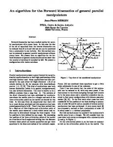
Figure 2: A typical phi-curve (φ in degree) only fives equatons among the six defined by equations (2) and therefore we have to verify that the links lengths associated to this solution are identical to the initial set. In order to verify the validity of one solution we define a performance index C: C=

6 X

||ρsi − ρi ||

(8)

1

where ρsi denotes the length of link i for a possible solution. This index will vanished for each solution of the forward kinematics. By the use of a discretization of φ we are able to get a plotting of C as a function of φ which is called a φ-curve. Figure 2 presents a typical φ-curve . By looking at the φ-curve we can determine among the possible solutions those which have a performance index close to zero. These solutions are then fed to a least square algorithm which enables to get the exact solutions. For example if we consider the φ-curve described in the figure we may seen that 4 solutions have an index close to zero. Taking into account the symmetrical solutions we will thus have 8 solutions for this particular case. Furthermore it can be shown that the discretization of φ has not to be done between [0, 2π] but only between [0, π] because any solution between [π, 2π] will give identical solutions to those find in the interval [0, π].

4

Particular cases

The previous section does not deal with particular cases for which the determinant of the system S vanishes. First we consider the case where sin θ = 0. In this case ρ12 is linear in term of x0 . Then ρ34 becomes linear in term of y0 . By using this results ρ26 can be written as z02 + c = 0. Thus we get two possible solutions and have only to verify if the corresponding links lengths are the same as the original set. If sin ψ(yb3 − yb2 ) = − sin φ(ya3 − ya2 ) then equation ρ65 does not contain any term in z0 . It is possible to show that the φ-curve will be identical if we choose any other equation instead of ρ65 . 4

Thus the only change compared with the general case is that we use another equation to compute the value of z0 . If sin ψ = sin φ = 0 then ρ12 is linear in term of x0 . Then ρ24 , ρ65 are linear in term of y0 , z0 . We expand ρ21 and if we define x = tan θ2 we get a fourth order polynomial in x. Thus we get a four possible solutions and have only to verify if the corresponding links lengths are the same as the original set.

5

Maximum number of solutions

Let us consider the two equations (6). We define x = tan ψ2 ,y = tan φ2 , z = tan 2θ . Then it can be shown that these equations are of order 6 and 10 in term of x, y, z. Consider now the general equation: (9) ρ21s (ψ, θ, φ) = ρ21 It can be written as: a4 cos4 θ + a3 cos3 θ + a2 cos2 θ + a1 cos θ + a0 = 0

(10)

where the coefficients ai are independent from θ. From equation (6) we deduce: cos θ = −

u2 u1

(11)

Substituting this value in equations (10),(7) yield to polynomials in x, y whose order are respectively 32 and 11. By calculating the resultant of the two polynomials we will get a polynomial which order will be at most 352 (32 x 11) and therefore there is at most 352 possible solutions for the forward kinematics of this parallel manipulator.

6

Numerical example

The following algorithm has been implemented: 1)verify if the initial set of links lengths can satisfied the particular cases. 2)compute the performance index C for a discretization of φ in the range [0, π]. 3)if C is sufficiently low use the possible solution as an estimate for a least-square method. This algorithm has been used for a manipulator with the following characteristics: number 0 2 3

xa -7 10 2

ya 10 7 -10

xb -2 6 4

yb 7 -1 -3

The initial set of links lengths is determined for the configuration x0 = 1, y0 = 2, z0 = 10, ψ = 10, θ = 20, φ = 30. The eight solutions are given in table 1.

7

Conclusion

The proposed algorithm enables to find all the solutions of the forward kinematics problem even in the case of non-polyhedral parallel manipulator. Its main drawback is that the computation time is rather important (about thirty seconds on a SUN 3-60 workstation). However many improvements can be made to simplify the computation.

5

x0 1.0 4.253603 -1.802148 -3.165565 -3.165565 -1.802148 4.253603 1.0

y0 2.0 1.212795 4.346853 0.707157 0.707157 4.346853 1.212795 2.0

z0 10.0 6.867130 5.755688 4.248109 -4.248109 -5.755688 -6.867130 -10.0

ψ 10.0 1.127391 286.858708 66.626576 66.626576 286.858708 1.127391 10.0

θ 20.0 63.026008 -68.123310 -73.802803 73.802803 68.123310 -63.026008 -20.0

φ 30.0 56.207058 140.5 19.714532 19.714532 140.5 56.207058 30.0

Table 1: Solution of the forward kinematics problem (all the angles are in degree)

6

References [1] Bricard R. ”M´emoire sur la th´eorie de l’octa`edre articul´e”, Journal de Math´ematiques pures et appliqu´ees, Liouville, cinqui`eme s´erie, tome 3, 1897 [2] Charentus S., Renaud M. ”Calcul du mod`ele g´eom´etrique direct de la plate-forme de Stewart”, LAAS Report n◦ 89260, 1989, July, Toulouse, France. [3] Gosselin. C. Kinematic analysis, optimization and programming of parallel robotic manipulators, Ph. D. thesis, McGill University, Montr´eal, Qu´ebec, Canada, 1988 [4] Hunt K.H. Kinematic geometry of mechanisms, Clarendon Press, Oxford, 1978 [5] Hunt K.H. ”Structural kinematics of in Parallel Actuated Robot Arms”. Trans. of the ASME, J. of Mechanisms,Transmissions, and Automation in design Vol 105: 705-712. [6] Merlet J-P. ”Parallel manipulators, Part 1, Theory” Rapport de Recherche INRIA n◦ 646, March 1987 [7] Merlet J-P. ”Force-feedback control of parallel manipulators” IEEE Int. Conf. on Robotics and Automation, Philadelphia,24-29 April 1988 [8] Merlet J-P. ”Parallel manipulators, Part 4, Mode d’assemblage et cin´ematique directe sous forme polynomiale” INRIA Research Report n◦ 1135, December 1989 [9] Nanua P., Waldron K.J. ”Direct kinematic Solution of a Stewart Platform”, IEEE Int. Conf. on Robotics and Automation, Scotsdale, Arizona, May 14-19 1989,pp. 431-437. [10] Reboulet C., Robert A. ”Hybrid control of a manipulator with an active compliant wrist”, 3th ISRR, Gouvieux,France, 7-11 Oct. 1985, pp. 76-80. [11] Stewart D. ”A platform with 6 degrees of freedom”,Proc. of the institution of mechanical engineers 1965-66, Vol 180, part 1, n◦ 15, pp.371-386.

7