Direct Kinematics and Assembly Modes of Parallel Manipulators - Inria

Direct Kinematics and Assembly Modes of Parallel Manipulators J-P. Merlet INRIA 2004 Route des Lucioles 06565 Valbonne Cedex, France E-mail : [email protected]

Abstract In this article we address the problem of the direct kinematics of parallel manipulators and the corollary problem of their assembly modes (i.e., the different ways of assembling these mechanisms when their geometry are fixed). As an example we consider first a 6-DOF manipulator with a triangular mobile plate and variable links lengths. A geometric proof is presented to show that the number of assembly modes is at most 16. Then we show that solving the direct kinematics problem is equivalent to solve a 16th-order polynomial in one variable, which is presented. We exhibit one example for which there are effectively 16 assembly modes. We extend then the results of this example to various architectures of parallel manipulators with a triangular mobile plate (among them the famous Stewart platform). Unfortunately the method used in those cases cannot be extended to the most general parallel manipulators. We introduce a more general approach and we present the results of this method on a particular case.

1

Introduction

Each articular coordinate ρi of a parallel manipulator can be expressed in general as a non linear function Fi of the generalized coordinates X of the end-effector (Merlet 1989a). We have: ρi = Fi (X)

i ∈ [1, n]

(1)

where n is the number of articular coordinates. The direct kinematics problem of a manipulator is addressed as follows: for a set of articular coordinates, determine the generalized coordinates of the effector i.e., solve the system of n non linear equations (1). We consider a parallel manipulator called the Triangular Symmetric Simplified Manipulator (TSSM) (see Figure 2)(Fichter 1986, Koliskor 1986), which is composed of an hexagonal base plate and a triangular mobile plate linked by six variable-length links. In that special case the links are articulated with the base plate through universal joints whose centers are coplanar and with the mobile plate through balland-socket joints whose centers are also coplanar. Hunt (1983) has proposed a conjecture that states that the number of assembly modes for the TSSM cannot be greater than 16. Nanua and Waldron (1989) have then shown that the direct kinematics problem for the TSSM can be reduced to the resolution of a 24th order polynomial in one variable. Such a result gives an upper bound of the number of assembly modes (called UBAM in the following sections), which is the degree of the polynomial. We will call such a polynomial the equivalent polynomial of the manipulator. Charentus and Renaud (1989) have proved that it is possible to find an equivalent polynomial for the TSSM whose degree is 16. 1

In a first part we prove the conjecture of Hunt and present the method to obtain the equivalent polynomial of the TSSM. We exhibit a configuration for which there are effectively 16 assembly modes. In a second part we generalize the approach used for the TSSM. This enables us to determine an UBAM for various architectures with a triangular mobile plate proposed in the literature (among them the famous Stewart platform), together with their equivalent polynomials. Finally, we consider a manipulator for which both the mobile and base plates are hexagonal and propose a UBAM and an equivalent polynomial.

2 2.1

The TSSM Equivalent mechanism

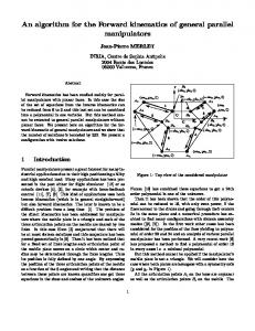
The TSSM (Figure 2) is a 6-DOF parallel manipulator in which a mobile plate is connected to a fixed base through six articulated links, each link being connected both at the base and at the mobile plate through ball-and-socket and universal joints. By controlling the links lengths we are able to control the position and orientation of the mobile plate (Zamanov 1984, Mohamed 1985, Reboulet 1985, Fichter 1986). In the following part we will use the notation defined in Fig. 1. The links are numbered from 1 to 6, and the center of the articulation on the base (mobile) of link i (whose length is ρi ) is denoted Ai (Bi ). We attach a reference frame O, x, y, z to the base and a mobile frame C, x1 , y1 , z1 to the mobile plate. The coordinates of Ai in the reference frame are (xai , yai , zai ), and the coordinates of Bi in the mobile frame are (xbi , ybi , zbi ). The coordinates of C in the reference frame are xc , yc , zc , and a posture of the mobile plate is defined by xc , yc , zc and the three Euler’s angle, ψ, θ, φ. The articulation points being coplanar, we may choose the position of O, C such that zai = zbi = 0. The distance between B3 and B5 is denoted by m, and the distance between B1 and B3 or B5 is defined as mp. We may notice that points A1 , A2 , B1 lie in a plane denoted P 12. In the same way, points A3 , A4 , B3 lie in the plane P 34 and points A5 , A6 , B5 in the plane P 56. We denote by p12 , p34 , p56 the angles between the planes P 12, P 34, P 56 and the base plane. For fixed link lengths the articulation points B1 , B3 , B5 of the mobile plate lie on circles centered in O12 , O34 , O56 whose radius are r12 , r34 , r56 (see Fig. 1). The centers and radii of these circles are fully determined by the link lengths. Thus the TSSM is equivalent to a mechanism constituted of three links articulated on coplanar revolute joints and connected to the mobile plate through ball-and-socket joints (Fig. 2). This mechanism is called the equivalent mechanism of the TSSM.

2.2

Determination of the Equivalent Polynomial

We consider the following three equations: ||B1 B3 ||2 − mp2 = 0

||B1 B5 ||2 − mp2 = 0

||B3 B5 ||2 − m2 = 0

(2)

If we denote by nij the unit vector between Oij and the corresponding articulation point on the mobile we have: OB1 = OO12 + r12 n12

OB3 = OO34 + r34 n34

OB5 = OO56 + r56 n56

(3)

Thus we get: B1 B3 B1 B5

= OO34 + r34 n34 − OO12 − r12 n12 = OO56 + r56 n56 − OO12 − r12 n12

(4) (5)

B3 B5

= OO56 + r56 n56 − OO34 − r34 n34

(6)

where OO12, OO34 , OO56 , r12 , r34 , r56 are fully determined by the known link lengths. As for n12 , n34 , n56 , they can be expressed as a function of the three unknown angles p12 , p34 , p56 . Therefore

2

equations (4)-(6) can be written as functions of these angles. It is possible to show (Merlet 1989b) that these equations may be written as: K11 sin(p34 ) sin(p12 ) + (K21 cos(p34 ) + K22 ) cos(p12 ) + K32 cos(p34 ) + K33 L11 sin(p56 ) sin(p12 ) + (L21 cos(p56 ) + L22 ) cos(p12 ) + L32 cos(p56 ) + L33

= =

0 0

(7) (8)

M11 sin(p34 ) sin(p56 ) + (M21 cos(p34 ) + M22 ) cos(p56 ) + M32 cos(p34 ) + M33

=

0

(9)

where the coefficients K, L, M do not depend on the angles p12 , p34 , p56 . It may be noticed that for a given set p12 , p34 , p56 , solution of the above equations, the set −p12 , −p34 , −p56 will also be a solution. This means simply that for a given posture of the mobile plate its reflection through the base has the same link lengths. Equations (7), (8) are linear in term of sin(p12 ), cos(p12 ). Solving this linear system and writing the identity equation cos(p12 )2 + sin(p12 )2 = 1 yield to: (N1 − N2 ) cos(p56 )2 + N5 sin(p56 ) + (N3 sin(p56 ) + N4 ) cos(p56 ) + N2 + N6 = 0

(10)

where the coefficients N are functions of p34 only. We get then the value of sin(p56 ) from equation (9): sin(p56 ) = −

(M21 cos(p34 ) + M22 ) cos(p56 ) + M32 cos(p34 ) + M33 M11 sin(p34 )

(11)

Using this value, equation (10) may be written as : I1 cos(p56 )2 + I2 cos(p56 ) + I3 = 0

(12)

The identity equation sin(p56 )2 + cos(p56 )2 = 1 is derived from equation (11) and is written as: H1 cos(p56 )2 + H2 cos(p56 ) + H3 = 0

(13)

The Ii , Hj coefficients are second order polynomials in cos(p34 ) only. The equivalent polynomial of the TSSM is obtained as the resultant of equations (12) and (13), defined by: |I1 H2 | |I1 H3 | (|Ii Hj | = Ii Hj − Ij Hi ) (14) |I1 H3 | |I2 H3 | = 0 The |Ii Hj | terms are fourth-order polynomials in cos(p34 ). Therefore, equation (14) is an eighth-order 2 ) polynomial in cos(p34 ). If we define x = tan( p234 ) we have cos(p34 ) = (1−x (1+x2 ) , and equation (14) becomes a 16th-order polynomial in x. In fact the coefficients of the odd power of x in this polynomial are all zero (this means that if p34 is a solution of the polynomial, −p34 is also a solution, as known from the beginning) and therefore we have to solve only an eighth-order polynomial. To solve the direct kinematics problem we first calculate p34 from the equivalent polynomial and then follow the method of Nanua and Waldron (1989) to determine the values of p12 , p56 . From the values of p12 , p34 , p56 it is easy to calculate the postures of the mobile plate. It must be noticed that the order of the polynomial is such that it is not possible to find its analytical solutions, but numerous numerical algorithms can be used in order to find its roots.

2.3

Example

We present here an example of a TSSM with 16 assembly modes (i.e., the equivalent polynomial has 16 real roots). The positions of the articulation points are given in Table 1. The link lengths are obtained for the posture xc = yc = 0, zc = 20, ψ = −10◦ , θ = −5◦ , φ = 10◦ . This yields to: ρ1 = 15.860466 ρ2 = 16.035246 ρ3 = 15.267173 ρ4 = 16.20915

ρ5 = 16.062666 3

ρ6 = 15.239395

The postures corresponding to the above link lengths are given in Table 2. We present in Figure 3 a drawing of the equivalent polynomial in order to show the necessary numerical accuracy. For that example we have used a grid of the working area to get the repartition of the number of assembly modes given in Table 3. Figure 4 shows the eight postures of the mobile plate for which the mobile plate is over the base.

2.4

Minimal degree of the TSSM Equivalent Polynomial

Following the reasoning of Hunt (1983), we will prove geometrically that there is at most 16 assembly modes for a TSSM. If we dismantle one of the link of the equivalent mechanism of the TSSM we get an RSSR mechanism (Fig. 5). It is known (Hunt 1978) that point B of this mechanism describes a 16th-order surface, the RSSR spin surface. The configurations of the mobile plate of the TSSM are determined by the intersection points of this surface, with the circle described by the extremity of the dismantled link. A 16th-order surface is intersected by a circle in no more than 32 points. Hunt assumes that the RSSR spin surface contains the imaginary spherical circle eight times and therefore deduces that at least 16 points are imaginary, yielding at most 16 assembly modes for the TSSM. Thus, to demonstrate this conjecture we have to determine the circularity of the RSSR spin surface. We give the outline of the calculation, described with more details in Merlet (1989b). Basically its principle is similar to the one used for the determination of the equivalent polynomial. First we define the coordinates of B in the reference frame as (X, Y, Z). We express the coordinates of B1 , B2 as a function of the angles p12 , p34 and write that the distances between the couple of points (B, B1 ), (B, B2 ), (B1 , B2 ) are constant. We get three equations that can be written as : E1 cos(p12 ) + E2 sin(p12 ) + E3 = 0

(15)

F1 cos(p34 ) + F2 sin(p34 ) + F3 = 0 K11 sin(p34 ) sin(p12 ) + (K21 cos(p34 ) + K22 ) cos(p12 ) + K32 cos(p34 ) + K33 = 0

(16) (17)

where the Ei , Fj coefficients do not depend on the angles, but only on the three coordinates of B. Equations (15)(17) are linear in term of sin(p12 ), cos(p12 ). We solve this linear system, and the result is used to write the identity equation cos(p12 )2 + sin(p12 )2 = 1. This yields: (N1 − N2 ) cos(p34 )2 + N3 sin(p34 ) cos(p34 ) + N4 sin(p34 ) + N5 cos(p34 ) + N6 + N2 = 0

(18)

Then sin(p34 ) is determined using equation (16). Putting the result in equation (18) and writing the identity equation sin(p34 )2 + cos(p34 )2 = 1 yields two equations: I1 cos(p34 )2 + I2 cos(p34 ) + I3 = 0 2

H1 cos(p34 ) + H2 cos(p34 ) + H3 = 0

(19) (20)

where the coefficients Ii , Hj are functions only of the coordinates of B. The resultant of these equations is a 16th-order polynomial whose higher degree term is: U 4 (Y 2 + X 2 + Z 2 )8 V 2 ,

(21)

where U, V are non zero constants. Therefore the circularity of the RSSR spin surface is 8 and the conjecture of Hunt is verified.

3

Equivalent Mechanisms

The equivalent mechanism of the TSSM, whose revolute joint axes are coplanar is called the equivalent mechanism of type 1. In the following parts we will consider various equivalent mechanisms that do not satisfy the constraint of coplanarity of the revolute joint axes. We will first consider the equivalent 4

mechanism with concurrent revolute joint axes (which intersection point is at infinity if the revolute joint axes are parallel)(Fig. 6). These mechanisms will be called the equivalent mechanisms of type 2. Finally, we will consider the general case where the revolute joint axis are in a general position (Fig. 7). This mechanism will be called the equivalent mechanism of type 3. In all cases we suppose we know the direction of the revolute joint axis, the position of the center of the revolute joint (with respect to some reference frame), the lengths of the three links, and the geometry of the mobile plate. Our purpose is to determine for this set of parameters what may be the three unknown revolute joint angles, together with the maximum number of solutions. For this last point we may state that in every case an UBAM is 16. Our proof uses the same method as the one used for the TSSM. In each case an RSSR mechanism is obtained by dismantling one link of the equivalent mechanism. The order of the RSSR spin surface is 16, and the solutions of the problem lie on the intersection of this surface with the circle on which lies the extremity of the dismantled link. This means that there will be at most 32 intersection points. However we have shown in Merlet (1989b) that the circularity of the RSSR spin surface is always 8, which means that there are at most 16 real intersection points. As for the determination of the solutions, Innocenti and Parenti-Castelli (1990) have shown recently that it is possible to get a 16th-order equivalent polynomial for any of the equivalent mechanism.

4 4.1

Case-by-Case Study of Parallel Manipulators 3-DOF Manipulators

We consider the mechanism described in Fig. 8(1), which has been studied by Gosselin (1988) and Lee and Shah (1988). This manipulator has three links with variable lengths, with one extremity of each link being connected to the base by a revolute joint and the other one to the mobile plate through a ball-and-socket joint. It is in fact the equivalent mechanism of type 1 and therefore has at most 16 assembly modes, and its direct kinematics can be expressed as a polynomial of order 8. Let us consider now the mechanism described in Figure 8(2). For this manipulator the link lengths are fixed but the position of the articulation points near the base can move along a vertical axis, the mobile plate being articulated on a ball-and-socket joint whose center is fixed in the reference frame: therefore this manipulator is a 3-DOF rotational wrist. A prototype of such a manipulator is currently under development in our laboratory under the direction of D. Simon. For a set of fixed articular coordinates (i.e., for a fixed position of A1 , A2 , A3 ) the articulation points of the mobile plate Bi may describe a circle centered on the line joining the center of the articulation point Ai and the center M of the ball-andsocket joint. Thus the equivalent mechanism of this manipulator is of type 2 (a). Consequently we may have only 16 different solutions. But the solutions lying under the base must be rejected as the mobile plate is constrained to be over the base by the articulation at M . Therefore an UBAM for this kind of architecture is 8, and we may find an equivalent polynomial of degree 16. In the case of our prototype, for which the base and mobile plates are equilateral triangles of radius 7 and 5, the link lengths and the height of the foot being 12, we have been able to find configurations with up to eight assembly modes. The Euler’s angles of the eight postures are given in Table 4, and the configurations are presented in Figure 9. We have investigated the repartition of the number of assembly modes in the working area (Table 5).

4.2 4.2.1

6-DOF manipulators The New INRIA Prototype

After having developed a ”left hand” (Merlet 1989a), our purpose was to design a new parallel manipulator that will be used as an active wrist. This yields to important constraints on the weight and on the position of the center of mass of the manipulator. Furthermore we wish to have a faster manipulator with an

5

increased working space, especially for the rotation. We have thus developed a new design, shown in Fig. 10. The mobility is ensured by moving the articulation points Ai of fixed-length links along a vertical direction. Thus the heavy part of the manipulator is near the base, and therefore the center of mass is very low. By using new linear actuators using a ball-screw and samarium-cobalt DC torque motors we get low mass, low friction, and fast actuators. The working space is increased because of the mechanical architecture, and there are fewer intersection problems with the links, which are thin aluminium beams. For a fixed position of the articular coordinates (i.e., for a fixed position of the Ai ), the articulation points Bj of the mobile may describe circles whose centers lie on the line joining the articulation centers Aj , Aj+1 of the corresponding links. The centers of these circles, together with their radii, can be determined according to the values of the articular coordinates. Therefore the manipulator equivalent mechanism is of type 3, with 16 as an UBAM and a 16th-order equivalent polynomial. For our prototype, whose link lengths are 10 and whose articulations points positions are given in Table 6, we have been able to find sets of articular coordinates such that there are up to 16 assembly modes.

4.3

Stewart Platform

This famous manipulator (Stewart 1965) is presented in Fig. 11. In this mechanism two rams (denoted l1 and l2 ) are articulated through revolute joints on a beam that can rotate around a vertical axis. The other extremity of ram l1 is connected to the mobile plate; ram l2 allows changes in the orientation of ram l1 . For fixed lengths of the six rams, the articulation points of the mobile plate can only rotate around a vertical axis (the beam axis), and thus the equivalent mechanism of the Stewart platform is of type 2b. Therefore the UBAM is 16, and we may find an equivalent polynomial of degree 16. For the Stewart platform defined by Table 7, we have been able to find sets of articular coordinates yielding to up to eight assembly modes. An example of such configurations is given in Table 8, and the postures are described in Figure 12. The repartition of the number of assembly modes in the working area is given in Table 9.

4.4

Others 6-DOF Manipulators With a Triangular Mobile Plate

Many other mechanical architectures have been proposed in the literature. Hunt (1983) describes a manipulator with fixed link length for which the articulation points near the base move along circles (Fig. 13). In this case it is easy to show that the equivalent mechanism is of type 3, and therefore the UBAM is 16. Han et al. (1989) define an architecture with fixed link lengths for which the articulation points near the base are connected to the coupler of four-bars mechanisms (see Figure 13). The equivalent mechanism is of type 1, but for a given input angle of the four-bars mechanism, there are two positions of the coupler and therefore at most 26 x16 = 1024 possible assembly modes. Kohli et al. (1988) uses in his manipulator linear-rotary actuators (see Figure 13), and we can see that the equivalent mechanism of this robot is of type 1, yielding to up to 16 assembly modes.

5

Manipulators With Hexagonal Plates

The method proposed for the manipulators with a triangular mobile plate is strongly dependent on the fact that the number of unknowns can be reduced easily from six to three (the three angles defining the orientation of the planar faces of the manipulator). Consequently this method cannot deal with a manipulator without planar faces or having no equivalent mechanism. An example of such a manipulator, called a Simplified Symetric Manipulator (SSM), is presented in Fig. 14: basically this manipulator is similar to the TSSM, but the mobile plate is a hexagon, with the centers of the articulation points of the mobile plate being coplanar. Furthermore, we assume that the hexagonal base and mobile plates have a symmetry axis. 6

We give the outline of a method to calculate the solutions of the direct kinematics problem; this method is described with more details in Merlet (1990). If we consider a link of the SSM, we may write the vector AB as: AB = AO + OC + CB = AO + OC + RCBr , (22) where CBr is the coordinate vector of B expressed in the mobile frame, and R is the rotation matrix between the mobile frame and the reference frame. The link length ρ can therefore be written as: ρ2

= ||AB||2 =

AOAOT + CBr CBr T + 2(AOT + CBr T RT )OC +2AOT RCBr + OCOCT

(23)

We notice that in the above equation the quadratic part in terms of the coordinates of C is OCOCT . Thus by substracting the square of two link lengths, we will get a linear equation in terms of these coordinates. If we define ρij as: ρij = ρ2i − Fi2 (X) − ρ2j + Fj2 (X) then the equations: ρ12 = 0

ρ45 = 0

ρ65 = 0

constitute a linear system in the three unknowns xc , yc , zc . This system is solved and the result reported in equations ρ24 = 0, ρ36 = 0. These equations can be written as: u1 cos θ + u2 = 0

v1 cos θ + v2 = 0

(24)

where u1 , u2 , v1 , v2 do not depend on θ. From the initial set of six equations, one remaining equation is: ρ21 = F12 (ψ, θ, φ)

(25)

a4 cos4 θ + a3 cos3 θ + a2 cos2 θ + a1 cos θ + a0 = 0

(26)

This equation can be written as:

where ai does not depend on θ. Using equation (24) we determine the value of cos θ, which is reported in equation (26). If we define x = tan( ψ2 ), y = tan( φ2 ) equation (26) becomes a 32nd-order polynomial in x, y. From equations (24) we deduce a new equation by u1 v2 − u2 v1 = 0

(27)

which is also polynomial in x, y whose degree is 11. The direct kinematics problems is reduced to the resolution of the system of equations (26) and (27). The resultant of these two equations gives the equivalent polynomial of the SSM whose degree (and therefore an UBAM of the SSM) is at most 11 x 32 =352. A numerical algorithm has been implemented, and we have found an SSM with up to twelve assembly modes. It must be noticed that, like for the TSSM, the reflection of a given posture through the base has the same link lengths. Figure 15 presents a set of configurations for which the mobile plate is over the base.

6

Conclusion

From this study we deduce that in general an UBAM of the 6-DOF parallel manipulator with triangular mobile plate is 16. We have presented a method that enables us to solve the direct kinematics problem by finding a polynomial in one variable whose roots determine the posture of the mobile plate. For the TSSM, a numerical resolution of this polynomial has proved that some sets of articular coordinates may effectively yield to sixteen postures. Because of the high degree of the equivalent polynomials and the

7

fact that their numerical resolution yields a great number of solutions, it seems that this approach is not usable for finding the analytical solution of the direct kinematic problem. The method presented for parallel manipulators with a triangular mobile plate cannot be extended to the more general case of parallel manipulators in which the mobile and base plates are both general hexagons. We have briefly presented a method that enables us to find an UBAM together with an equivalent polynomial for the special case in which the articulation points on each plate are coplanar. It must still be understood why the duality between serial and parallel manipulators is so complete; indeed for the resolution of the inverse kinematic problem of serial manipulators (which is the dual problem of the direct kinematics problem of parallel manipulators) Raghavan and Roth (1989) have established that one has to solve a 16th-order polynomial. The similitude between both problems is sufficiently appealing that we hope to find an explanation for this duality.

References []

Charentus, S. and Renaud, M. 1989,(Montr´eal, June 19-21). Modelling and control of a modular, redundant robot manipulator. 1st Int. Symp. on Experimental Robotics.

[]

Fichter, E.F. 1986. A Stewart platform based manipulator: General theory and practical construction.Int. J. Robot. Res. 5(2):157-181.

[]

Gosselin, C. 1988. Kinematic analysis, optimization and programming of parallel robotics manipulators. Ph.D. thesis, McGill University, Montr´eal, Qu´ebec, Canada.

[]

Han, C.-S., Tesar, D., and Traver, A. 1989 (Montr´eal, May). The optimum design of a 6 dof fully parallel micromanipulator for enhanced robot accuracy. ASME Design in Automation Conf., pp. 357-363.

[]

Hunt, K.H. 1978. Kinematic Geometry of Mechanisms. Oxford: Clarendon Press.

[]

Hunt, K.H. 1983 Structural kinematics of in parallel actuated robot arms. Trans. ASME J. Mechanisms Transmissions Automation Design. (105):705-712.

[]

Innocenti, C. and Parenti-Castelli, V. 1990 Direct position analysis of the Stewart platform mechanism. Mechanism Machine Theory 25(6):611-621.

[]

Kohli, D., Lee , S.-H., Tsai, K.-Y., and Sandor, G.N. 1988. Manipulator configurations based on rotary-linear (R-L) actuators and their direct and inverse kinematics. J. Mechanisms Transmissions Automation Design 110:397-404.

[]

Koliskor, A. Sh. 1986 (Suzdal, April 22-25). The l-coordinate approach to the industrial robot design. V IFAC/IFIP/IMACS/IFORS Symposium, pp. 108-115.

[]

Lee, K-M. and Shah, D.K. 1988. Kinematic analysis of a three-degrees-of-freedom in-parallel actuated manipulator. IEEE J. Robot. Automation 4(3):354-360.

[]

Merlet, J-P. 1989a. Manipulateurs parall`eles. 3eme partie: Applications. INRIA research report no. 1003.

[]

Merlet, J-P. 1989b. Manipulateurs parall`eles. 4eme partie: d’assemblage. INRIA research report no. 1135.

[]

Merlet, J-P. 1990. An algorithm for the forward kinematics of general 6-DOF parallel manipulators. INRIA research report no. 1331.

[]

Mohamed, M.G. and Duffy, J. 1985. A direct determination of the instantaneous kinematics of fully parallel robot manipulators. Trans. ASME J. Mechanisms Transmissions Automation Design 107:226-229. 8

Cin´ematique directe et mode

[]

Nanua, P. and Waldron, K.J. 1989 (Scotsdale, AZ, May 14-19). Direct kinematic solution of a Stewart platform. IEEE Int. Conf. on Robotics and Automation,pp. 431-437.

[]

Raghavan, M. and Roth, B. 1989 (Tokyo, Aug. 28-31). Kinematic analysis of the 6r manipulator of general geometry. 5th Int. Symp. of Robotics Research, pp. 314-320.

[]

Reboulet, C. and Robert, A. 1985 (Gouvieux, France, Oct. 7-11). Hybrid control of a manipulator with an active compliant wrist. Proc. 3rd ISRR, pp. 76-80.

[]

Stewart, D. 1965-1966. A platform with 6 degrees of freedom. Proc. Inst. Mech. Engineers 1801(15):371-386.

[]

Zamanov, V.B and Sotirov, Z.M. 1984 (Tokyo, July 11-13). Structures and kinematics of parallel topology manipulating systems. Proc. Int. Symp. on Design and Synthesis, pp. 453-458.

9

a B1 a12 O12

A1 1

A6

A2

r12

2

mp 6

y1 C x

O

a56

A1 , A2 B3

B5

a34

P 56

m

B5

r56

base

3 x1

B3

P 12

p12

A3

B1

y

P 34

O34 p56

ap

4

5

O56

r34

base

base

p34

A5 , A6

g

A3 , A4

A4

A5

Figure 1: Notation. The TSSM is represented in top view.

B1 mobile

B5

link

articulations

B3 r34

r12

r56 p56

O12

p34 O34

O56 base

Figure 2: The TSSM parallel manipulator and its equivalent mechanism.

point A1 A2 A3 A4 A5 A6

xa -9.7 9.7 12.76 3.0 -3.0 -12.76

base ya 9.1 9.1 3.9 -13.0 -13.0 3.9

point za 0.0 0.0 0.0 0.0 0.0 0.0

xb

mobile yb

zb

B1

0.0

7.3

0.0

B3

4.822

-5.480722

0.0

B5

-4.822

-5.480722

0.0

Table 1: Positions of the articulation points on the base and the mobile plate for the TSSM with 16 assembly modes (see Figure 1 for the location of the Ai , Bj ).

10

y: polynomial value

0

y: polynomial value 0.0000682

-0.0571937

0.0000132 0

-0.1144045

-0.0000417

-0.1716153

-0.0000967

-0.2288261

-0.0001516

abscissa:p34 (degree) y: polynomial value

p34 (degree)

p34 (degree) -0.0002066

-0.2860368 0.00 0.0009265

8.28

16.68

25.08

33.48

42 0.0573176

y: polynomial value

42.00 y

43.97

62.00

66.53

45.97

47.97

49.97

75.73

80.33

0.0361935

0.0002501 0 -0.0004264

0.0150695

-0.0011028

0 -0.0060546

-0.0017792

-0.0271787 p34 (degree)

-0.0024557

52.00

53.97

55.97

57.97

59.97

-0.0483027

p34 (degree) 71.13

Figure 3: Equivalent polynomial associated to the TSSM with 16 assembly modes. It may be seen that this polynomial effectively has 8 real roots.

11

xc 0.0 -1.413449 1.361778 0.160610 0.109944 2.802948 -2.335532 -0.352493 -0.352493 -2.335532 2.802948 0.109944 0.160610 1.361778 -1.413449 0.0

yc 0.0 4.826228 4.903809 5.376522 -6.807134 -4.666035 -4.467979 -3.866344 -3.866344 -4.467979 -4.666035 -6.807134 5.376522 4.903809 4.826228 0.0

zc 20.0 17.42996 17.38246 17.186792 15.157245 12.740689 12.547885 11.918376 -11.918376 -12.547885 -12.740689 -15.157245 -17.186792 -17.38246 -17.42996 -20.0

ψ -10 102.640488 -106.331771 -170.380852 178.790092 55.389531 -50.849043 -12.559631 167.440521 129.151104 -124.610623 -1.210054 9.619302 73.668386 -77.359662 -10

θ -5 147.384474 149.931849 164.013963 104.247298 89.178208 79.039617 45.110726 45.110726 79.039617 89.178208 104.247298 164.013963 149.931849 147.384474 5

φ 10 -61.976868 58.9676 7.954509 -179.39757 136.199674 -137.353267 -168.301331 11.698826 42.64689 -43.800473 0.602583 -172.045644 -121.032543 118.023282 10

Table 2: The sixteen postures of the TSSM for which the link lengths are identical (the angles are in degree).

Figure 4: Example of 8 over-the-base assembly modes of a TSSM with identical link lengths (perspective, top, and side view).

12

number of solutions %

2 0.6927

4 26.04269

6 10.5282

8 45.209

10 3.9559

12 10.6

14 1.0945

16 1.876

Table 3: Repartition of the number of assembly modes in the working area of the TSSM with 16 assembly modes (grid of 297381 points, xc , yc : ±8, zc ∈ [19 − 21], ψ, θ, φ : ±15◦ ).

B

B2

B1

Figure 5: The RSSR mechanism obtained when one link of the equivalent mechanism of the TSSM is dismantled.

a) b)

Figure 6: Equivalent mechanisms with concurrent and parallel revolute joint axes: the equivalent mechanism of type 2.

case 1 2 3 4

ψ -145.0 -154.035628 -85.964358 34.035628

θ 0.0 136.277574 136.277574 136.277574

case 5 6 7 8

φ 0.0 42.982182 77.017821 -42.982186

ψ -34.035639 85.964344 154.035656 25.2

θ 136.277574 136.277574 136.277574 0.0

φ -77.017814 162.982179 -162.982179 0.0

Table 4: Three rotational degrees of freedom INRIA prototype: eight configurations with identical articular coordinates (Euler’s angles, in degrees).

13

B1 B5

l12

l56 p12

p56

B3 p34 l34

Figure 7: Equivalent mechanism of type 3.

A2

A1

M 1

2 A3

Figure 8: 3-DOF parallel manipulator (1) and parallel manipulator with three rotational degrees of freedom (INRIA prototype) (2).

solutions %

1 1.575

2 73.51

3 2.42

4 12.62

5 2.29

6 4.057

7 1.183

8 2.039

Table 5: Repartition of the number of assembly modes in the working area for the 3 rotational DOF INRIA prototype (grid of 13777 points).

14

1

5

6

2

8 3

7 4

Figure 9: Eight assembly modes of the three rotational degrees of freedom INRIA prototype (perspective, top, and side view; angles in degrees).

point A1 A2 A3 A4 A5 A6

base xa ya -5.5 4.33 5.5 4.33 6.5 2.6 1.0 -6.93 -1.0 -6.93 -6.5 2.6

point

mobile xb yb

zb

B1

0.0

4.0

0.0

B3

3.464

-2.0

0.0

B5

-3.464

-2.0

0.0

Table 6: Positions of the articulation points on the base and the mobile plate for the INRIA prototype with 16 assembly modes.

15

double ball-and-socket joint B3

B1

B5

A4 A2

A3 A5

A6 A1 universal joint

base

Figure 10: The new INRIA prototype and its mechanical architecture.

point A1 A2 A3 C1 C2 C3

xa -17.32 17.32 0 -17.32 17.32 0

base ya 10 10 -20 10 10 -20

point za 5 5 5 10 10 10

mobile xb yb

zb

B1

-4.32

2.5

0.0

B2

4.32

2.5

0.0

B3

0

-5

0.0

Table 7: Definition of the position of the articulation points for a Stewart platform with 8 assembly modes. The dead length of l1 is 5.

16

C3 A3 B3 B2 l1

C2

B1 C1

l2 A2

A1

Figure 11: Stewart platform.

17

xc -0.954574 1.342928 0.107103 -5.648898 -5.002486 0 5.127337 4.029389

yc 5.98857 5.488324 0.257609 -2.640058 -3.505835 0 -1.195835 -3.638017

zc 10 10 10 10 10 10 10 10

ψ -70.793887 -23.016429 -30.023243 -160.420740 177.103960 130 41.343222 95.780739

θ 160 160 20 160 160 20 160 160

φ 130 130 130 130 130 130 130 130

Table 8: Eight assembly modes of a Stewart platform (angles in degree).

x = −0, 954 y = 5, 99 z = 10 ψ = −70, 79 θ = 160 φ = 130

x = −5 y = −3, 5 z = 10 ψ = 177, 1 θ = 160 φ = 130

x = 1, 342 y = 5, 488 x = 0 y = 0 z = 10 z = 10

ψ = −23, 016 θ = 160 φ = 130

ψ = 130 θ = 20 φ = 130

x = 5, 127 y = −1, 198 z = 10 ψ = −30, 023 θ = 20 φ = 130 x = 0, 107 y = 0, 257 z = 10 ψ = 41, 34 θ = 160 φ = 130

x = −5, 6489 y = −2, 64 z = 10

x = 4, 03 y = −3, 638 z = 10

ψ = 177, 1 θ = 160 φ = 130

ψ = 95, 78 θ = 160 φ = 130

Figure 12: Eight assembly modes of a Stewart platform (perspective, side, and top view; angles in degrees).

18

solutions %

1 8.500

2 83.957

3 0.578

4 5.619

5 0.456

6 0.752

7 0.0385

8 0.09

Table 9: Repartition of the number of assembly modes of a Stewart platform in its working area (grid of 15552 points). []

[]

[]

Figure 13: 6-DOF parallel manipulators. C

A6

x

mobile

6 A1

B6 5

SSM A6

base

O A4

A3

B1

C

A4 A5

1 B5

A5

B4 4

B3

2 3

A1

y B2

A3

A2

A2

Figure 14: A 6-DOF parallel manipulator without planar faces: the SSM. 1

4

5

2

3

6

Figure 15: Six configurations of a SSM for which the link lengths are identical (perspective, top, and side view). The six other postures are the reflections through the base plate of these configurations. 19

List of Figures 1 2 3 4 5 6 7 8 9 10 11 12 13 14 15

Notation. The TSSM is represented in top view. . . . . . . . . . . . . . . . . . . . . . . . The TSSM parallel manipulator and its equivalent mechanism. . . . . . . . . . . . . . . . Equivalent polynomial associated to the TSSM with 16 assembly modes. It may be seen that this polynomial effectively has 8 real roots. . . . . . . . . . . . . . . . . . . . . . . . Example of 8 over-the-base assembly modes of a TSSM with identical link lengths (perspective, top, and side view). . . . . . . . . . . . . . . . . . . . . . . . . . . . . . . . . . . The RSSR mechanism obtained when one link of the equivalent mechanism of the TSSM is dismantled. . . . . . . . . . . . . . . . . . . . . . . . . . . . . . . . . . . . . . . . . . . Equivalent mechanisms with concurrent and parallel revolute joint axes: the equivalent mechanism of type 2. . . . . . . . . . . . . . . . . . . . . . . . . . . . . . . . . . . . . . . Equivalent mechanism of type 3. . . . . . . . . . . . . . . . . . . . . . . . . . . . . . . . . 3-DOF parallel manipulator (1) and parallel manipulator with three rotational degrees of freedom (INRIA prototype) (2). . . . . . . . . . . . . . . . . . . . . . . . . . . . . . . . . Eight assembly modes of the three rotational degrees of freedom INRIA prototype (perspective, top, and side view; angles in degrees). . . . . . . . . . . . . . . . . . . . . . . . The new INRIA prototype and its mechanical architecture. . . . . . . . . . . . . . . . . . Stewart platform. . . . . . . . . . . . . . . . . . . . . . . . . . . . . . . . . . . . . . . . . . Eight assembly modes of a Stewart platform (perspective, side, and top view; angles in degrees). . . . . . . . . . . . . . . . . . . . . . . . . . . . . . . . . . . . . . . . . . . . . . . 6-DOF parallel manipulators. . . . . . . . . . . . . . . . . . . . . . . . . . . . . . . . . . A 6-DOF parallel manipulator without planar faces: the SSM. . . . . . . . . . . . . . . . Six configurations of a SSM for which the link lengths are identical (perspective, top, and side view). The six other postures are the reflections through the base plate of these configurations. . . . . . . . . . . . . . . . . . . . . . . . . . . . . . . . . . . . . . . . . . .

10 10 11 12 13 13 14 14 15 16 17 18 19 19

19

List of Tables 1 2 3 4 5 6 7 8 9

Positions of the articulation points on the base and the mobile plate for the TSSM with 16 assembly modes (see Figure 1 for the location of the Ai , Bj ). . . . . . . . . . . . . . . . The sixteen postures of the TSSM for which the link lengths are identical (the angles are in degree). . . . . . . . . . . . . . . . . . . . . . . . . . . . . . . . . . . . . . . . . . . . . . Repartition of the number of assembly modes in the working area of the TSSM with 16 assembly modes (grid of 297381 points, xc , yc : ±8, zc ∈ [19 − 21], ψ, θ, φ : ±15◦ ). . . . . . Three rotational degrees of freedom INRIA prototype: eight configurations with identical articular coordinates (Euler’s angles, in degrees). . . . . . . . . . . . . . . . . . . . . . . . Repartition of the number of assembly modes in the working area for the 3 rotational DOF INRIA prototype (grid of 13777 points). . . . . . . . . . . . . . . . . . . . . . . . . . . . Positions of the articulation points on the base and the mobile plate for the INRIA prototype with 16 assembly modes. . . . . . . . . . . . . . . . . . . . . . . . . . . . . . . . . . . Definition of the position of the articulation points for a Stewart platform with 8 assembly modes. The dead length of l1 is 5. . . . . . . . . . . . . . . . . . . . . . . . . . . . . . . . Eight assembly modes of a Stewart platform (angles in degree). . . . . . . . . . . . . . . Repartition of the number of assembly modes of a Stewart platform in its working area (grid of 15552 points). . . . . . . . . . . . . . . . . . . . . . . . . . . . . . . . . . . . . .

10 12 13 13 14 15 16 18 19