Backward vs. Forward-oriented Decision Making in the Iterated Prisoner’s Dilemma: A Comparison between Two Connectionist Models Emilian Lalev1 and Maurice Grinberg1 1
Central and East European Center for Cognitive Science, New Bulgarian University, 21 Montevideo Street, 1618 Sofia, Bulgaria
[email protected],
[email protected]
Abstract. We compare the performance of two connectionist models developed to model specific aspects of the decision making process in the Iterated Prisoner’s Dilemma Game. Both models are based on common recurrent network architecture. The first of them uses a backward-oriented reinforcement learning algorithm for learning to play the game while the second one makes its move decisions based on generated predictions about future games, moves and payoffs. Both models involve prediction of the opponent move and of the expected payoff and have an in-built autoassociator in their architecture aimed at more efficient payoff matrix representation. The results of the simulations show that the model with explicit anticipation about game outcomes could reproduce the experimentally observed dependence of the cooperation rate on the so-called cooperation index thus showing the importance of anticipation in modeling the actual decision making in human participants. The role of the models’ building blocks and mechanisms is investigated and discussed and a comparison with experiments with human subjects are presented.
Keywords: anticipation, cooperation, decision-making, recurrent artificial neural network, reinforcement learning.
1 Introduction In formal game theory players are described as perfectly rational and possessing perfect information about the game including not only their possible moves and payoffs but also those of their opponents. On the other hand, the bounded rationality view on cognition states that people are almost never perfectly rational (see e.g. [1]). Moreover, they try to minimize the cognitive effort while making decisions. Finally, the results of experiments involving games demonstrate that people rarely play as prescribed by the normative game theory. We have started a series investigations on the cognitive processes involved in decision making in Iterated Prisoner’s Dilemma Game (IPDG) from a cognitive science point of view [2-5] using different approaches involving psychological experiments, eye-tracking experiments, and modeling and simulations.
2 In ref. [3], a simple model based on expected subjective utility theory was put forward. The model used extensively backward reinforcement learning mechanisms and based on that made predictions about the move probability of the opponent. Additionally in order to explain some specific characteristics of the decision making process explicit accounting of the current game was added. The latter allowed for the description of the well known dependence of the cooperation rate and the structure of the payoff matrix expressed by the so called Cooperation Index (CI) (see ref. [6]). This property is not available in typical reinforcement learning based models used to model playing of IPDG and in which the probability for cooperation is based only on past games (see refs. [7-8]). Taking into account the results obtained by Hristova and Grinberg [3], here we propose a connectionist architecture based on a recurrent network which accounts for the payoff structure of the PD game, the past moves and payoffs and predicts the next moves of the player and his/her opponent, and the expected payoff from the next game. A related attempt, using recurrent neural networks, to model the complexity of IPDG have been made by Taiji and Ikegami [10] but in their model only the moves of the players are used in the recurrent network and only a single payoff matrix is played, so the question of the influence of the different ratios among the payoffs in different game matrices (i.e. dependence on game CI) could not be considered. Further two variants based on the general architecture were explored. The first involved training of the next-move output node using a backward looking reinforcement model (see ref [9] for details), further referred to as Model B. In the second, the training of the move node was based on evaluation of the future payoffs and thus essentially using anticipation (further referred to as Model A). The analysis and comparisons of the simulation results of the two models with recent experimental results and the discussion of the importance of the mechanisms involved are the main concern of this paper. 1.1 The Prisoner’s Dilemma Game The Prisoner’s dilemma is a two-person game. The payoff table for this game is presented in Table 1.The players simultaneously choose their move – ‘C’ (cooperate) or ‘D’ (defect), without knowing their opponent’s choice. Table 1. Payoff table for the PD game. In each cell the comma separated payoffs are the Player I’s and Player II’s payoffs, respectively.
Player I
Player II C
D
C
R, R
S, T
D
T, S
P, P
2
3 In Table 1, R is the payoff if both players cooperate (play ‘C’), P is the payoff if both players ‘defect’ (play ‘D’), T is the payoff if one defects and the other cooperates, S is the payoff if one cooperates and the other defects. The payoffs satisfy the inequalities T > R > P > S and 2R > T + S. This structure of the payoff matrix of that game offers a dilemma to the players: there is no obvious best move. The dominant ‘D’ move (T>R and P>S) would lead to lower payoffs if adopted by all the players (payoff P) although this is the choice prescribed by standard game theory. Cooperation seems to be the best strategy in the long run (R>P) but at the risk of one of the opponents to start to defect and the other to receive the lowest payoff S. Rapoport and Chammah [6] proposed the quantity CI = (R–P)/(T–S), called cooperation index, as a predictor of the probability of ‘C’ choices, monotonously increasing with CI. In Table 2 two examples of PD games with different CI − 0.1 and 0.9, respectively − are presented. Table 2. Examples of PD game matrices with different CI – 0.1 and 0.9, respectively. The first payoff in each cell is the payoff of the ‘row’ player and the second of the ‘column’ player. Player II C D
C
56, 56
0, 60
D
60, 0
50, 50
CI=0.9 Player I
Player I
CI=0.1
Player II C D
C
56, 56
0, 60
D
60, 0
2, 2
This quite complicated situation is at the heart of the dilemma in this game and is the reason for the on-going interest in this game over the past 50 years and continuing today. From a cognitive modeling point of view the challenge is to understand the decision making mechanisms that would lead to the results observed in the experiments with human participants taking account of all characteristics (like the dependence on CI for instance). We are convinced that the models needed must have a minimal level of complexity and account for playing based on the payoff matrix of the game (e.g. to be sensitive to CI) and on the opponent moves and game outcomes. In the same time human players rely on past experience and predictions of future events. The models presented here are aimed at complying with these requirements
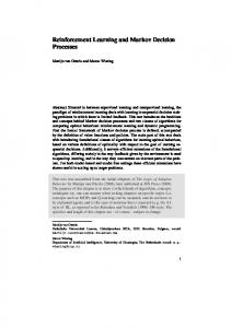
2 Models – Architectures and Functioning 2.1 Basic Architecture The core architecture (underlying both presented models) is an Elman recurrent neural network [11] (see Fig. 1). In ref. [10], a recurrent network has also been used to model the behaviour of PD game players. However, the network we used has a much more complicated structure to include in the network input/output structure the game payoff matrices, the players’ moves and the received payoffs (related to the specific game outcome). The network consists of eight input, thirty hidden-layer, and six out-
3
4 put nodes (see Fig. 1). The activation functions of the hidden layer and of the output layer are tan-sigmoid and log-sigmoid functions, respectively. Because of the logistic output activation function, a part of the network’s outputs could be interpreted as probabilities. 2.1.1 Inputs and Outputs All the inputs of the network were rescaled within the range [0, 1]. As can be seen in Fig. 1, the values of the payoffs from the current game matrix (excluding the payoff S which was always 0), as well as the past game payoff received, the player’s and opponent’s moves in the previous game were presented at the input nodes at each cycle.
Fig. 1. Schematic view of the recurrent neural network and its inputs and outputs/targets. Notation: Sm and Cm are respectively the simulated subject and computer opponent (probability for) moves; Poff(t) is the player’s received payoff at time t.
The past moves were recoded as [0,1] – for ‘C’ and [1,0] – for ‘D’ moves, so that activation would always come from any of the two couples of input nodes, no matter what the moves were – ‘C’ or ‘D’. The values of the T, R, and P payoffs from the current game had to be reproduced as an output by the model thus implementing an in-built autoassociator. There were two reasons to decide to include this component in the network architecture. The first was that this would force the network to establish representations of the games in its hidden layer which is crucial to account for the game payoff structure in the decision making process. The second one was related to the anticipatory decision mechanism of Model A where the output nodes concerning T, R, and P were used as predictions of the next games’ payoffs (see Section 2.2.2 for details). At the output, the player’s move (‘Sm’ node) and the computer-opponent’s move (‘Cm’ node) nodes were interpreted as the probability for cooperation for the player and the prediction about the probability of cooperation of his/her opponent in the game at hand. The payoff (‘Poff’) node represented the expected gain from the current game.
4
5 2.1.2 Training PD games with varying CI – from 0.1 to 0.9 – were presented to the neural network (T was always equal to 1, and S was always 0, R and P were distributed in this interval depending on the CI of a particular game). The games were randomized with respect to CI in the same way as in the experiments with human participants (see e.g. [2,3]) in order to allow comparison with the experimental results (see Section 3). The network was trained using back-propagation on an input consisting of sequences of overlapping five games – the current game and the four previous games. Such sequences are further called micro-epochs. In the very beginning of the IPDG, the length of micro-epochs was increasing with each next completed game until it reached five games. The very first inputs were as follows: the first game matrix, the player’s move and the prediction of the opponent’s move generated with probability 0.5. The first received payoff (Poff) was obtained from the averaging of the payoffs of the games. The small number of games, the network dealt with at a time, implies sensitivity to local changes in the game and to memory constraints we assumed to exist in real game playing. On the other hand, the micro-epochs were long enough so that specific events in the history of IPDG were able to encode in the memory of the recurrent hidden layer. The values at the six output nodes were used as predictions when the network was trained within the current micro-epoch. The ‘T’, ‘R’, and ‘P’ output nodes were expected to reproduce the corresponding input values in the input payoff matrices. The output of the ‘Sm’ node was the model-player’s probability for cooperation in the current game. The output at the node ‘Cm’ was the prediction for the cooperation probability of the opponent, and the output at the ‘Poff’ node meant the expected game payoff. When both player and opponent had made their moves, and the payoff for the model-player is known, the new target micro-epoch was updated and the network was trained with the inputs it was simulated with and the new targets. For all of the output nodes the training signal is supplied by the game (payoffs) and the opponent moves except for the model-player’s move probability. The latter has to be supplied either from experimental data with a human player (if the model is used to fit the behaviour of a real player) or by explicitly modeling the evaluation of the game outcome. Here, we will present results along the latter line based on two different choices of such an evaluation. 2.2 Decision Making of the Models In order to build a realistic model able to make decisions comparable to the ones made by human subjects, we needed to make an assumption for an evaluation mechanism for the outcomes of the player’s moves. Hereafter, we discuss two such mechanisms, both based on received payoff maximization, which differ in the emphasis on backward or forward evaluation.
5
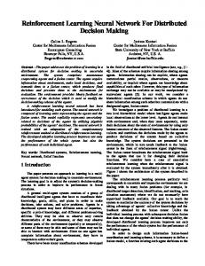
6 2.2.1 Backward-looking Model (Model B) Model B integrates the recurrent network presented in Section 2.1 with the Bush – Mosteller (BM) backward-looking reinforcement learning model in the form proposed by Macy and Flache in ref. [9]. We integrated the Macy and Flache model with our recurrent neural network by using the predicted payoff – ‘Poff(t)’ (see Fig. 1) as the player’s aspiration level and used it to estimate the target cooperation probability. The current move of the model was generated with a probability equal to the output at the ‘Sm’ node (see Fig. 1). After the game moves were made by the player and its opponent, and the player’s payoff was already known, a target probability was calculated using the Macy’s and Flache’s model [9]. The ‘Cm’ target node was trained using the actual opponent’s move and the ‘Poff’ output node using the received payoff. The latter was considered to be a kind of aspiration level based on payoff expectation and was used instead of the aspiration update rule from ref. [9]. As explained before, the ‘T’, ‘R’, and ‘P’ output nodes were trained using the values from the input game matrix as targets. This combination of a neural network model and a reinforcement model was expected to give a model player sensitive to specific game episodes in IPDG and to the payoffs in the game matrix at hand (which could give rise to a CI dependent strategy). Theoretically, when the model encountered an episode, in which all predictions, except for the move prediction) resembled those from any past episode, it would play with a similar cooperation probability from that past episode. The dynamics of the decision making process is illustrated in Fig. 2, where the fluctuation of the aspiration level together with the player’s move probability are shown. It is seen from Fig. 2 that as expected low aspiration level leads to high probability of cooperation because the payoffs R are above the aspiration level. M ov e 'C' probability and Aspiration - mode l B 1
0,6 0,4
level
0,8
0,2 0 1
14
27
40
53
66
79
92 105 118 131 144 157 170 183 196
Game numbe r 'C' probability
Aspiration
Fig. 2. Dynamics of aspiration (output ‘Poff’ node) and cooperation probabilities in Model B (‘Sm’ node).
2.2.2 Forward-looking Model (Model A) Model A is based on the same neural network architecture as Model B but is aimed at using essentially anticipation mechanisms for deciding about its moves. Model A uses the predictive properties of the recurrent network in order to “guess” how the game would proceed if its current move were either ‘C’ or ‘D’. An anticipatory module was implemented in the model, so that two sequences of five games pre-
6
7 dicted by the neural network were produced before making a move. The first sequence began with a ‘C’ move, and the second one with a ‘D’ move. Only the first player move was fixed in any sequence. The recurrent network had as first inputs the current game input (together with the other four games from the micro-epoch) including the values of the T, R, and P payoffs, and the players’ moves and payoff from the previous game. This is a simpler mechanism as the one used in ref. [10], where all the combinations of moves are taken into account. Here the first move is chosen and everything else is based on the network prediction. As the player move was known in the first fictitious game (‘C’ or ‘D’), the opponent move was generated with the probability predicted by the network. The payoff for the player from the game was calculated according to the rules of PD game – T, R, P or S based on the moves of both players. In the second fictitious game the input micro-epoch was updated so that the new T, R, and P values are taken from the output layer of the neural network and considered as prediction about the fictitious game payoffs. The ‘Poff(t-1)’ node activation got the value of the fictitious payoff from the previous game and the previous moves nodes (the ‘Sm(t-1)’ and ‘Cm(t-1)’ nodes) activations were the fictitious previous game moves. In the next iterations everything was repeated except for that the player move was generated with its predicted probability and was no longer fixed. So the cycle was closed and the model could predict several future games and related moves and outcomes. The payoffs from both sequences ( Poff C for initial move ‘C’ and Poff D for initial move ‘D’) were then considered. The obtained payoffs from the five fictitious games for each initial move choice were evaluated using a discount factor as follows: 5
Poff C , D = ∑ Poff C , D (t ) β t −1 ,
(1)
t =1
where Poff C , D (t ) is the value of the payoff at moment t , for initial move ‘C’ or ‘D’ and β is the usual discount parameter that indicated to what extend the remote future game payoffs were important for making decisions at present. If
β
was 0, only the
first fictitious payoff would matter, and if β was 1, all the payoffs would be considered as equally important. The probability for cooperation for the current move of the model was then calculated using a soft-max function:
P (C ) =
e Poff C / k , e Poff C / k + e Poff D / k
(2)
where P(C ) is the calculated cooperation probability and k is a parameter for the sensitivity of the function towards the difference between Poff C and Poff D . The smaller the value k had, the greater the sensitivity to the difference between the ‘C’ and ‘D’ alternative choices became.
7
8
3 Game Simulations 3.1 The Computer Opponent The models were run against a probabilistic Tit-for-two-Tats (Tf2T) computer strategy. Its move depended on the player’s two previous moves, thus being adaptive to their temporal cooperativeness without being easily predictable. Depending on the two previous opponent’s moves the probability for cooperation was respectively: 0.5 for ‘C, D’ and ‘D, C’, 0.8 for ‘C, C’, and 0.2 for ‘D, D’. Furthermore, the same computer opponent was used in a series of experiments and such a choice for the simulations here allows for a comparison with the experimental results (see Section 3.2). They both had the underlying recurrent neural network that provided them with the ability to “recognize” and predict events in the IPDG and, therefore, be able to extract important information such as the strategy of the opponent from the history of the game. Both made their moves probabilistically so that they had the chance to evoke different aspects of their adaptive opponent’s strategy, which might have remained invisible otherwise. 3.2 Comparison of Model and Experimental Results The results presented in this section are based on 30 IPDG sessions of two-hundred games against the Tf2T computer strategy for each model (B and A). For the comparisons with experiment the first 50 games are taken (to match the number of games played by human participants. From the experiment reported in ref. [2], only data for from the first part and for the control condition is used (see [2] for details). 30 participants played 50 PD games against the computer. The computer used the probabilistic Tf2T strategy described above. This was done to allow the subject to choose his/her own strategy without easily become aware of the computer-opponent’s strategy. The payoffs were presented as points, which were transformed into real money and paid at the end of the experiment. After each game the subjects got feedback about their and the computer’s choice and could monitor permanently the total number of points they have won and its money equivalent. The subjects received information about the computer’s payoff only for the current game and had no information about the computer’s total score. This was made to prevent a possible shift of subjects’ goal – from trying to maximize the number of points to trying to outperform the computer. In this way, the subjects were stimulated to pay more attention to the payoffs and their relative magnitude and thus indirectly to CI. The best fit of the experimental results was obtained with the following parameters were used for Model A (see eqs. (1) and (2)): β = 0.3 and k = 0.05. 3.3 Mean Cooperation and Payoffs In Model B’s performance, the payoffs were significantly correlated with the mean level of cooperation in contrast to Model A whose payoffs were not correlated with its cooperation rates against the Tf2T computer player. These results reflect the different
8
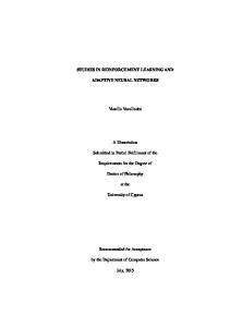
9 nature of the outcome evaluation mechanism – reinforcement learning for Model B and payoff anticipation for Model A. The results for the mean cooperation and payoffs for Model A, Model B, and human participants experimental data taken from ref. [2] are presented in Fig. 3. Regarding mean cooperation, only Model A and the experimental data were not statistically different (F= 0.121, p = 0.73). The mean cooperation was different for Model B and experiment (F=5.858, p=0.019) and for Model B and Model A (F=6.267, p=0.015). For the mean payoff no significant difference was found between simulations and experiment. Mean Rescaled Cooperation and Payoffs for Models A, B, and Experimental Subjects
mean rescaled value (0:1)
0,6 0,5 0,4 Model A 0,3
Model B Subjects
0,2 0,1 0 Mean Cooperation
Mean Payoff
Fig. 3. Comparison of mean cooperation and payoffs between Model A and B, and experimental data from human subjects (taken from ref. [2]).
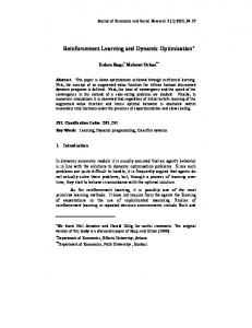
3.4 Dependence of Cooperation Rate on CI To start with a main effect of CI on cooperation rates was observed in Model A (F=16.908, p