Foundations of parallel algorithms PRAM model Time, work ... - IDA

FDA125 APP Lecture 2: Foundations of parallel algorithms.

1

¨ C. Kessler, IDA, Linkopings Universitet, 2003.

FDA125 APP Lecture 2: Foundations of parallel algorithms.

2

¨ C. Kessler, IDA, Linkopings Universitet, 2003.

Literature

Foundations of parallel algorithms

¨ Practical PRAM Programming. [PPP] Keller, Kessler, Traff: Wiley Interscience, New York, 2000. Chapter 2.

PRAM model Time, work, cost

[JaJa] JaJa: An introduction to parallel algorithms. Addison-Wesley, 1992.

Self-simulation and Brent’s Theorem Speedup and Amdahl’s Law

[CLR] Cormen, Leiserson, Rivest: Introduction to Algorithms, Chapter 30. MIT press, 1989.

NC Scalability and Gustafssons Law

[JA] Jordan, Alaghband: Fundamentals of Parallel Processing. Prentice Hall, 2003.

Fundamental PRAM algorithms reduction parallel prefix list ranking

PRAM variants, simulation results and separation theorems. Survey of other models of parallel computation Asynchronous PRAM, Delay model, BSP, LogP, LogGP FDA125 APP Lecture 2: Foundations of parallel algorithms. FDA125 APP Lecture 2: Foundations of parallel algorithms.

3

4

¨ C. Kessler, IDA, Linkopings Universitet, 2003.

¨ C. Kessler, IDA, Linkopings Universitet, 2003.

Parallel computation models (2)

Parallel computation models (1) + abstract from hardware and technology + specify basic operations, when applicable

Cost model: should + explain available observations + predict future behaviour

+ specify how data can be stored

! analyze algorithms before implementation independent of a particular parallel computer

! focus on most characteristic (w.r.t. influence on time/space complexity) features of a broader class of parallel machines Programming model

Cost model

shared memory vs. message passing

key parameters

degree of synchronous execution

constraints

cost functions for basic operations

+ abstract from unimportant details ! generalization Simplifications to reduce model complexity: use idealized machine model ignore hardware details: memory hierarchies, network topology, ... use asymptotic analysis drop insignificant effects use empirical studies calibrate parameters, evaluate model

5

FDA125 APP Lecture 2: Foundations of parallel algorithms.

¨ C. Kessler, IDA, Linkopings Universitet, 2003.

Flashback to DALG, Lecture 1: The RAM model

6

FDA125 APP Lecture 2: Foundations of parallel algorithms.

¨ C. Kessler, IDA, Linkopings Universitet, 2003.

The RAM model (2)

RAM (Random Access Machine)

[PPP 2.1]

programming and cost model for the analysis of sequential algorithms data memory .....

s = d(0) do i = 1, N-1 s = s + d(i) Example: Computing the global sum of N elements end do N t = tload + tstore + ∑ (2tload + tadd + tstore + tbranch) = 5N 3 2 Θ(N ) Algorithm analysis: Counting instructions

i=2

M[3]

s

M[2]

+ s

M[1] M[0]

+ s +

load clock

s

store

+ s program memory

CPU

+

ALU

+

register 1 current instruction

+

s +

+

s

register 2 ....

+

+

+

+

+

PC

d[0] d[1] d[2] d[3] d[4] d[5] d[6] d[7]

d[0] d[1] d[2] d[3] d[4] d[5] d[6] d[7]

! arithmetic circuit model, directed acyclic graph (DAG) model FDA125 APP Lecture 2: Foundations of parallel algorithms. FDA125 APP Lecture 2: Foundations of parallel algorithms.

7

8

¨ C. Kessler, IDA, Linkopings Universitet, 2003.

¨ C. Kessler, IDA, Linkopings Universitet, 2003.

PRAM model

[PPP 2.2]

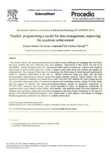
Parallel Random Access Machine

[Fortune/Wyllie’78]

PRAM model: Variants for memory access conflict resolution Exclusive Read, Exclusive Write (EREW) PRAM concurrent access only to different locations in the same cycle

p processors Concurrent Read, Exclusive Write (CREW) PRAM simultaneous reading from or single writing to same location is possible

MIMD common clock signal Shared Memory

arithm./jump: 1 clock cycle shared memory

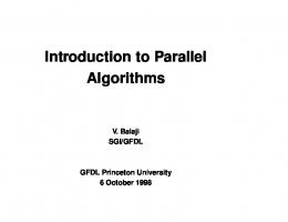
Concurrent Read, Concurrent Write (CRCW) PRAM simultaneous reading from or writing to same location is possible:

CLOCK

Weak CRCW

uniform memory access time latency: 1 clock cycle (!) concurrent memory accesses sequential consistency private memory (optional)

P 0 M0

P 1 M1

P 2 M2

P3 M3

......

Pp-1 Mp-1

?

Common CRCW Arbitrary CRCW

Shared Memory

a CLOCK

Priority CRCW Combining CRCW (global sum, max, etc.)

processor-local access only

P1

P2

P3

M0

M1

M2

M3

Mp-1

nop;

*a=0;

*a=2;

t: *a=0; *a=1;

No need for ERCW ...

......

P0

Pp-1

9

FDA125 APP Lecture 2: Foundations of parallel algorithms.

¨ C. Kessler, IDA, Linkopings Universitet, 2003.

10

FDA125 APP Lecture 2: Foundations of parallel algorithms.

Global sum computation on EREW and Combining-CRCW PRAM (1) Given n numbers x0; x1; :::; xn

1

¨ C. Kessler, IDA, Linkopings Universitet, 2003.

Global sum computation on EREW and Combining-CRCW PRAM (2)

stored in an array.

Recursive parallel sum program in the PRAM progr. language Fork [PPP]

The global sum ∑ xi can be computed in dlog2 ne time steps i=0 on an EREW PRAM with n processors. n 1

Parallel algorithmic paradigm used: Parallel Divide-and-Conquer d[0] d[1] d[2] d[3] d[4] d[5] d[6] d[7]

ParSum(n): +

ParSum(n/2)

+

+

+

ParSum(n/2) +

+ +

+

t

Divide phase: trivial, time O(1) Recursive calls: parallel time T (n=2) with base case: load operation, time O(1) Combine phase: addition, time O(1)

sync int parsum( sh int *d, sh int n) { sh int s1, s2; sh int nd2 = n / 2; if (n==1) return d[0]; // base case $=rerank(); // re-rank processors within group if ($ 1012.

TSM (n) TAM ( p; n)

=

parallelization slowdown of A: Is N C

=P

?

Hence, SUabs( p; n) =

For some problems in P no polylogarithmic PRAM algorithm is known ! likely that N C 6= P ! P -completeness [PPP p. 46]

31

TSM (n) TAN (n) Used in the 1990’s to disqualify parallel processing by comparing to newer superscalars absolute, machine-nonuniform speedup =

32

¨ C. Kessler, IDA, Linkopings Universitet, 2003.

¨ C. Kessler, IDA, Linkopings Universitet, 2003.

Scalability

Example: Cost-optimal parallel sum algorithm on SB-PRAM n = 10; 000 Processors Clock cycles Time SUrel Sequential 460118 1.84 1 1621738 6.49 1.00 4 408622 1.63 3.97 16 105682 0.42 15.35 64 29950 0.12 54.15 256 10996 0.04 147.48 1024 6460 0.03 251.04 Processors Clock cycles Sequential 4600118 1 16202152 4 4054528 16 1017844 64 258874 256 69172 1024 21868

TAM (1; n) TSM (n)

SUrel( p; n) SL(n)

FDA125 APP Lecture 2: Foundations of parallel algorithms. FDA125 APP Lecture 2: Foundations of parallel algorithms.

SL(n) =

For machine N with p  pA(n), SUabs

EF

0.28 1.13 4.35 15.36 41.84 71.23

1.00 0.99 0.96 0.85 0.58 0.25

n = 100; 000 Time SUrel SUabs 18.40 64.81 1.00 0.28 16.22 4.00 1.13 4.07 15.92 4.52 1.04 62.59 17.77 0.28 234.23 66.50 0.09 740.91 210.36

EF 1.00 1.00 0.99 0.98 0.91 0.72

we have tA( p; n) = O(cA(n)= p) and thus SUabs( p; n) = p

! linear speedup for cost-optimal A ! “well scalable” (in theory) in range 1  p  pA(n) ! For fixed n, no further speedup beyond pA(n)

TSM (n) . cNA (n)

For realistic problem sizes (small n, small p): often sublinear! - communication costs (non-PRAM) may increase more than linearly in p - sequential part may increase with p – not enough work available ! less scalable What about scaling the problem size n with p to keep speedup?

33

FDA125 APP Lecture 2: Foundations of parallel algorithms.

Isoefficiency

¨ C. Kessler, IDA, Linkopings Universitet, 2003.

[Rao,Kumar’87]

¨ C. Kessler, IDA, Linkopings Universitet, 2003.

Gustafssons Law

measured efficiency of parallel algorithm A on machine M for problem size n EF( p; n) =

34

FDA125 APP Lecture 2: Foundations of parallel algorithms.

TAM (1; n) SUrel( p; n) = M p p
TA ( p; n)

Let A solve a problem of size n0 on M with p0 processors with efficiency ε.

Revisit Amdahl’s law: assumes that sequential work As is a constant fraction β of total work. ! when scaling up n, wAs (n) will scale linearly as well! Gustafssons Law

[Gustafsson’88]

Assuming that the sequential work is constant (independent of n), given by seq. fraction α in an unscaled (e.g., size n = 1 (thus p = 1)) problem such that TAs = αT1(1), TA p = (1 α)T1(1), and that wA p (n) scales linearly in n, the scaled speedup for n > 1 is predicted by

The isoefficiency function for A is a function of p, which expresses the increase in problem size required for A to retain a given efficiency ε. If isoefficiency-function for A linear ! A well scalable Otherwise (superlinear): A needs large increase in n to keep same efficiency.

s SUrel (n)

=

Tn(1) Tn(n)

=

α + (1

α)n

=

n

(n

1)α:

The seq. part is assumed to be replicated over all processors.

FDA125 APP Lecture 2: Foundations of parallel algorithms.

35

¨ C. Kessler, IDA, Linkopings Universitet, 2003.

n=1:

s SUrel (n)

=

=

Tn(1) Tn(n)

1

P0

α T(1) 1 n>1:

reduction

(1−α) T(1) 1

P0 P1 P2 P3

s (n) SUrel

=

=

n

(n

1)α.

p see parallel sum algorithm

prefix-sums list ranking

Oblivious (PRAM) algorithm: [JaJa 4.4.1] control flow (! execution time) does not depend on input data.

Pn-1

α + (1 α)n 1

¨ C. Kessler, IDA, Linkopings Universitet, 2003.

n

TAs + wA p (n) TAs + TA p

assuming perfect parallelizability of A p up to p = n processors

36

Fundamental PRAM algorithms

Proof of Gustafssons Law

Scaled speedup for p = n > 1:

FDA125 APP Lecture 2: Foundations of parallel algorithms.

P0 P1 P2 P3

p

Oblivious algorithms can be represented as arithmetic circuits whose shape only depends on the input size.

P0 P1 P0

n (1−α) T(1) 1

Yields better speedup predictions for data-parallel algorithms.

Examples: reduction, (parallel) prefix, pointer jumping; sorting networks, e.g. bitonic-sort [CLR’90 ch. 28], ! Lab, mergesort Counterexamples: (parallel) quicksort

37

FDA125 APP Lecture 2: Foundations of parallel algorithms.

¨ C. Kessler, IDA, Linkopings Universitet, 2003.

38

FDA125 APP Lecture 2: Foundations of parallel algorithms.

The Prefix-sums problem

Sequential prefix sums computation

Given: a set S (e.g., the integers) a binary associative operator  on S, a sequence of n items x0; : : : ; xn 1 2 S

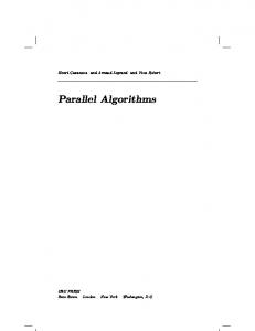
void seq_prefix( int x[], int n, int y[] ) { int i; int ps; // i’th prefix sum if (n>0) ps = y[0] = x[0]; for (i=1; inext != e) e->rank = 1; else e->rank = 0; nn = length; while (nn>1) { e->rank = e->rank + e->next->rank; e->next = e->next->next; nn = nn>>1; // division by 2 }

Every step + doubles #lists + halves lengths 5

¨ C. Kessler, IDA, Linkopings Universitet, 2003.

List ranking (2): Pointer jumping

Extended problem: compute the rank = distance to the end of the list Pointer jumping

6

46

4

3

FDA125 APP Lecture 2: Foundations of parallel algorithms.

2

1

47

! dlog2 ne steps

}

Not work-efficient!

Also for parallel prefix on a list!

¨ C. Kessler, IDA, Linkopings Universitet, 2003.

FDA125 APP Lecture 2: Foundations of parallel algorithms.

! Exercise 48

¨ C. Kessler, IDA, Linkopings Universitet, 2003.

CREW is more powerful than EREW

Simulating a CRCW algorithm with an EREW algorithm

Example problem: Given a directed forest, compute for each node a pointer to the root of its tree.

A p-processor CRCW algorithm can be no more than O(log p) times faster than the best p-processor EREW algorithm for the same problem. Step-by-step simulation

CREW: with pointer-jumping technique in dlog2 max. depthe steps e.g. for balanced binary tree: O(log log n); an O(1) algorithm exists EREW: Lower bound Ω(log n) steps per step, one given value can be copied to at most 1 other location e.g. for a single binary tree: after k steps, at most 2k locations can contain the identity of the root A Θ(log n) EREW algorithm exists.

[Vishkin’83]

For Weak/Common/Arbitrary CRCW PRAM: handle concurrent writes with auxiliary array A of pairs. CRCW processor i should write xi into location li: EREW processor i writes hli; xii to A[i] Sort A on p EREW processors by first coordinates in time O(log p) [Ajtai/Komlos/Szemeredi’83], [Cole’88] Processor j inspects write requests A[ j] = hlk ; xk i and A[ j 1] = hlq; xqi and assigns xk to lk iff lk 6= lq or j = 0. For Combining (Maximum) CRCW PRAM: see [PPP p.66/67]

FDA125 APP Lecture 2: Foundations of parallel algorithms.

49

¨ C. Kessler, IDA, Linkopings Universitet, 2003.

50

FDA125 APP Lecture 2: Foundations of parallel algorithms.

¨ C. Kessler, IDA, Linkopings Universitet, 2003.

Simulation summary

PRAM Variants

EREW  CREW  CRCW

Broadcasting with selective reduction (BSR) PRAM

Common CRCW  Priority CRCW

Distributed RAM (DRAM)

Arbitrary CRCW  Priority CRCW

Local memory PRAM (LPRAM)

[PPP 2.6]

Asynchronous PRAM where : “strictly weaker than” (transitive)

Queued PRAM (QRQW PRAM) Hierarchical PRAM (H-PRAM)

See [PPP p.68/69] for more separation results. Message passing models: Delay model, BSP, LogP, LogGP ! Lecture 4

FDA125 APP Lecture 2: Foundations of parallel algorithms.

51

¨ C. Kessler, IDA, Linkopings Universitet, 2003.

Broadcasting with selective reduction (BSR) BSR: generalization of a Combine CRCW PRAM

52

FDA125 APP Lecture 2: Foundations of parallel algorithms.

¨ C. Kessler, IDA, Linkopings Universitet, 2003.

Asynchronous PRAM [Akl/Guenther’89]

1 BSR write step:

Asynchronous PRAM SHARED MEMORY .......

Each processor can write a value to all memory locations (broadcast) Each memory location computes a global reduction (max, sum, ...) over a specified subset of all incoming write contributions (selective reduction)

[Cole/Zajicek’89] [Gibbons’89] [Martel et al’92]

store_sh load_sh

NETWORK P0

P1

P2

....... Pp-1 processors store_pr

M0 M1 M2

fetch&incr

atomic_incr

....... M p-1

private memory modules

No common clock No uniform memory access time Sequentially consistent shared memory

load_pr

FDA125 APP Lecture 2: Foundations of parallel algorithms.

53

¨ C. Kessler, IDA, Linkopings Universitet, 2003.

Delay model

FDA125 APP Lecture 2: Foundations of parallel algorithms.

54

¨ C. Kessler, IDA, Linkopings Universitet, 2003.

BSP model

Idealized multicomputer: point-to-point communication costs time tmsg.

Bulk-synchronous parallel programming

[Valiant’90] [McColl’93]

time

BSP computer = abstract message passing architecture ( p; L; g; s) time

MIMD

P0 P1 P2 P3 P4 P5 P6 P7 P8 P9

tw word transfer time

SPMD

global barrier t startup time s

Cost of communicating a larger block of n bytes:

time tmsg(n) = sender overhead + latency + receiver overhead + n/bandwidth =: tstartup + n
ttransfer

h-relation models communication pattern / volume

local computation using local data only

size

superstep

hi [words] = comm. fan-in, fan-out of Pi

communication phase (message passing) next barrier

Assumption: network not overloaded; no conflicts occur at routing

h = max1i p hi

tstartup = startup time (time to send a 0-byte message)

tstep = w + hg + L

accounts for hardware and software overhead

BSP program = sequence of supersteps, separated by (logical) barriers

ttransfer = transfer rate, send time per word sent depends on the network bandwidth.

FDA125 APP Lecture 2: Foundations of parallel algorithms. FDA125 APP Lecture 2: Foundations of parallel algorithms.

55

BSP example: Global maximum computation (non-optimal algorithm) Compute maximum of n numbers A[0; :::; n

56

¨ C. Kessler, IDA, Linkopings Universitet, 2003.

¨ C. Kessler, IDA, Linkopings Universitet, 2003.

1] on BSP( p; L; g; s):

// A[0::n 1] distributed block-wise across p processors step // local computation phase: m ∞; for all A[i] in my local partition of A f m max (m; A[i]); // communication phase: Local work: if myPID 6= 0 Θ(n= p) send ( m, 0 ); else // on P0: Communication: for each i 2 f1; :::; p 1g h= p 1 recv ( mi, i ); (P0 is bottleneck) step tstep = w + hg + L if myPID = 0 n  for each i 2 f1; :::; p 1g =Θ + pg + L m max(m; mi); p

LogP model (1) LogP model

[Culler et al. 1993]

for the cost of communicating small messages (a few bytes) 4 parameters: latency L overhead o gap g (models bandwidth) processor number P

g P0

o

send

g P1

abstracts from network topology

o

recv

L

gap g = inverse network bandwidth per processor: Network capacity is L=g messages to or from each processor. L, o, g typically measured as multiples of the CPU cycle time. transmission time for a small message: 2
o + L if the network capacity is not exceeded

time

57

FDA125 APP Lecture 2: Foundations of parallel algorithms.

¨ C. Kessler, IDA, Linkopings Universitet, 2003.

LogP model (2)

58

FDA125 APP Lecture 2: Foundations of parallel algorithms.

¨ C. Kessler, IDA, Linkopings Universitet, 2003.

LogP model (3): LogGP model

P0

P2 The LogGP model [Culler et al. ’95] extends LogP by parameter G = gap per word, to model block communication

P1

Example: Broadcast on a 2-dimensional hypercube

P3 Communication of an n-word-block:

With example parameters P = 4, o = 2µs, g = 3µs, L = 5µs 0

P0

1

send

2

3

4

5

6

send

P1

7

8

9

10

11

12

13

14

15

16

with the LogP-model: 17

18

Remark: gap constraint does not apply to recv; send sequences

sender

g o

g o

g o

g o

with the LogGP-model: o GGGG

g

o GGGG

recv send L

P2

receiver

recv

P3

L o

L o

L o

o

o

o

recv time

it takes at least 18µs to broadcast 1 byte from P0 to P1; P2; P3 tn = (n Remark: for determining time-optimal broadcast trees in LogP, see [Papadimitriou/Yannakakis’89], [Karp et al.’93] FDA125 APP Lecture 2: Foundations of parallel algorithms.

59

¨ C. Kessler, IDA, Linkopings Universitet, 2003.

Summary Parallel computation models Shared memory: PRAM, PRAM variants Message passing: Delay model, BSP, LogP, LogGP parallel time, work, cost Parallel algorithmic paradigms (up to now) Parallel divide-and-conquer (includes reduction and pointer jumping / recursive doubling) Data parallelism Fundamental parallel algorithms Global sum Prefix sums List ranking Broadcast

1)g + L + 2o

tn0 = o + (n

1)G + L + o