reusable way while constraining the use of the data by understanding what can ... ral and atemporal modelling constructors; this is usually realised by a ..... C1isaC2 or R1isaR2, respectively); Disjointness and Covering constraints over.
Foundations of Temporal Conceptual Data Models Alessandro Artale and Enrico Franconi Faculty of Computer Science, Free University of Bozen-Bolzano, Italy {artale,franconi}@inf.unibz.it
Abstract. This chapter considers the different temporal constructs appeared in the literature of temporal conceptual models (timestamping and evolution constraints), and it provides a coherent model-theoretic formalisation for them. It then introduces a correct and succinct encoding in a subset of first-order temporal logic, namely DLRU S – the description logic DLR extended with the temporal operators Since and Until. At the end, results on the complexity of reasoning in temporal conceptual models are presented.
1
Introduction
Conceptual data models describe an application domain in a declarative and reusable way while constraining the use of the data by understanding what can be drawn from it. A number of conceptual modelling languages has emerged as de facto standards; in particular, we mention entity-relationship (ER) for the relational data model, UML and ODMG for the object-oriented data model, and RDF and OWL for the web ontology languages. We consider here conceptual modelling languages able to represent dynamic and evolving information in the context of temporal databases [21, 26, 27, 32, 33, 38–40]. We provide in this chapter a mathematical foundation for them by summarising the various efforts appeared in the literature [4, 7, 23, 34, 35]. The main temporal modelling constructs we analyse can be distinguished in two main categories, timestamping and evolution constraints. To support timestamping, the data model should distinguish between temporal and atemporal modelling constructors; this is usually realised by a temporal marking of classes, relationships and attributes that translates into a timestamping mechanism in the corresponding database. A data model supports evolution constraints if it is able to keep track of how the domain elements evolve along time. In particular, status classes describe how elements of classes change their status from being a potential member till they cease forever to be member of the class; transitions deal with the fact that an object may migrate from one class to another one; while generation constraints describe processes that are responsible for the creation/disappearance of objects from classes. The formalisation is based on a model-theoretic semantics that captures the meaning of both timestamping and evolution constraints. The semantics is obtained as a temporal extension of the model-theoretic semantics associated to A.T. Borgida et al. (Eds.): Mylopoulos Festschrift, LNCS 5600, pp. 10–35, 2009. c Springer-Verlag Berlin Heidelberg 2009 �
Foundations of Temporal Conceptual Data Models
11
conceptual models [14, 18]. The advantage of associating a set-theoretic semantics to a language is not only to clarify the meaning of the language constructors but also to give a semantic definition to relevant modelling notions. In particular, we are able to give a rigorous definition to the notions of: schema satisfiability – when a schema admits a non empty interpretation which guarantees that the constraints expressed by the schema are not contradictory; class and relationships satisfiability – when a class or a relation admits at least an interpretation in which it is not empty; logical implication when a new (temporal) constraint is necessarily true in a schema even if not explicitly mentioned; and finally the special case of logical implication involving subsumption between classes (resp. relationships) – when the interpretation of a class (resp. relationship) is necessarily a subset of the interpretation of another class (resp. relationship). Building on the provided model-theoretic semantics we provide a correspondence between temporal conceptual models and logical theories expressed in a fragment of first order temporal logic, namely as a Description Logics (DLs) theory. DLs allow for the logical reconstruction and the extension of conceptual models (see [9, 14, 19]). The advantage of using a DL to formalise a conceptual data model lies basically on the fact that complete logical reasoning can be employed using an underlying DL inference engine to verify a conceptual specification, to infer implicit facts and stricter constraints, and to manifest any inconsistencies during the conceptual design phase. In addition, given the high complexity of the modelling task when complex data are involved, there is the demand for more sophisticated and expressive languages than for normal databases. Again, DL research is very active in providing more expressive languages for conceptual modelling (see [13, 14, 17, 18, 18, 19, 24, 31]). In this context, we consider the temporal description logic DLRU S [5], a combination of the expressive and decidable description logic DLR [17] (a description logic with n-ary relationships) with the linear temporal logic with temporal operators Since (S) and Until (U) which can be used in front of both classes and relations. We use DLRU S both to capture the temporal modelling constructors in a succinct way, and to use reasoning techniques to check satisfiability, subsumption and logical implication. The mapping towards DLs presented in this chapter builds on top of a mapping which has been proved correct in [3, 4] while complexity results and algorithmic techniques can be found in [1, 5, 11]. Even if full DLRU S is undecidable we address interesting modelling scenarios where subsets of the full DLRU S logic is needed and where reasoning becomes a decidable problem. The chapter is organised as follows. Section 2 describes the temporal constructs that will be the subject of the formalisation. Section 3 shows the modelling requirements that lead us to elaborate the rigorous definition of the framework presented here. Section 4 introduces the model-theoretic semantics and the notions of satisfiability, subsumption and logical implication for temporal conceptual models. The two Sections 5, 6 are the core sections where we describe how timestamping and evolution constraints can be formalised. After presenting the DLRU S logic in Section 7 we proceed with a DLRU S encoding of the
12
A. Artale and E. Franconi PaySlipNumber(Integer) Name(String)
Member S
S mbr
S
Salary(Integer)
T
Employee S
emp
Works-for T
org
act
(1,n)
ProjectCode(String)
OrganizationalUnit
Manager T
S
(3,n)
Project (1,1)
d
Department S
prj InterestGroup
AreaManager
TopManager
man (1,1)
Manages
Fig. 1. The Company example
various temporal constructs in Section 8. Section 9 investigates the complexity of reasoning over temporal conceptual models and presents various scenarios where sound, complete and terminating procedures can be used. In Section 10 we state our final remarks.
2
Temporal Modelling Constructors
Temporal constructs are usually added to the classical constructs to capture the temporal behaviour of the different components of a conceptual schema. In this chapter we distinguish them in two generic classes: Timestamping and Evolution constructs. Timestamping. It is concerned with the discrimination at the schema level between those elements of the model that change over time and others that are time invariant. Timestamping applies to classes, relationships and attributes. Data models should allow for both temporal and atemporal modelling constructors. Timestamping for attributes allows keeping how an attribute of a given object changes over time. For example (see Figure 1), the salary of an employee emp-123 has value “2.5K $” for the period from 01/2004 to 12/2005, then “3.0K $” from 01/2006 to 12/2007, then “3.2K $” from 01/2008 to 12/2009. Similarly, temporal periods can characterise an object or relationship instance as a whole rather than through its attributes. Membership in a class (relationship) can be characterised as limited in time or, vice versa, global— possibly modelling legacy classes (relationships). For example, the company schema (Figure 1) models the membership of objects in the Employee class as time-invariant while objects in the Manager class have a limited lifespan as member of that class. Timestamping is the basis for associating the notion of lifecycle [37] to the object/relationship instances as members of a given class/relationship (more details are given in Section 6.1). Section 5 shows how evolution constraints can be formalised.
Foundations of Temporal Conceptual Data Models
13
Evolution Constraints. They control the mechanism that rules dynamic aspects, i.e., what are the permissible transitions from one state of the database to the next one [6, 7, 22, 38]. When applied to classes we talk about Object Migration, i.e., the evolution of an object from being member of a class to being member of another class [29]. For example, an object in the Employee class may migrate to become an object of the Manager class or an object of the AreaManager class can evolve into a TopManager class. When object migration combines with timestamping we talk about Status Classes. In this case we specify constraints on the membership of an object in a class by splitting it into periods according to a given classification criterion. For example, existence of a manager object in the Manager class can include periods where the object is an active member of the class (e.g., the manager is currently on payroll), periods where its membership is suspended (e.g., the manager is on temporary leave), and a period where its membership is disabled (e.g., the manager has left the company) [22]. The notion of status for classes allows also for a fine grained notion of lifecycle which can now depend on the membership to a particular status of a class. Evolution-related knowledge may be conveyed also through relationships. Generation relationships [28] between objects of class A and objects of class B (possibly equal to A) describe the fact that objects in B are generated by objects in A. For example, in a company database, the splitting of a department translates into the fact that the original department generates two (or more) new departments. Clearly, if A and B are temporal classes, a generation relationship with source A and target B entails that the lifecycle of a B object cannot start before the lifecycle of the related A object. This particular temporal framework, where related objects do not coexist in time, is a form of, so called, across-time relationships [7, 38]. Section 6 shows how timestamping can be formalised. In the conceptual modelling literature, different notion of ’time’ have been considered. Notably, the most relevant distinction is between the so called valid time—which is the time when a property holds, i.e., it is true in the representation of the world—and transaction time—which records the history of database states rather than the world history, i.e., it is the time when a fact is current in the database and can be retrieved. In the following, we will consider both timestamping and evolution constructs as ranging over the valid time dimension.
3
Modelling Requirements
This Section briefly illustrates the requirements that are frequently advocated in the literature on temporal data models when dealing with temporal constraints [34, 38]. – Orthogonality. Temporal constructors should be specified separately and independently for classes, relationships, and attributes. Depending on application requirements, the temporal support must be decided by the designer. – Upward Compatibility. This term denotes the capability of preserving the non-temporal semantics of conventional (legacy) conceptual schemas when embedded into temporal schemas.
14
A. Artale and E. Franconi
– Snapshot Reducibility. Snapshots of the database described by a temporal schema are the same as the database described by the same schema, where all temporal constructors are eliminated and the schema is interpreted atemporally. Indeed, this property specifies that we should be able to fully rebuild a temporal database by starting from the single snapshots. These requirements are not so obvious when dealing with evolving objects. The formalisation carried out in this chapter provides a data model able to respect these requirements also in presence of evolving objects. In particular, orthogonality affects mainly timestamping [37] and our formalisation satisfies this principle by introducing temporal marks that could be used to specify the temporal behaviour of classes, relationships, and attributes in an independent way (see Section 5). Upward compatibility and snapshot reducibility [34] are strictly related. Considered together, they allow to preserve the meaning of atemporal constructors. In particular, the meaning of classical constructors must be preserved in such a way that a designer could either use them to model classical databases, or when used in a genuine temporal setting their meaning must be preserved at each instant of time. We enforce upward compatibility by using global timestamps over legacy constructors (see Section 5). Snapshot reducibility is hard to preserve when dealing with generation relationships where involved object may not coexist. We enforce snapshot reducibility by a particular treatment of relationship typing (see Section 6.3).
4
A Formalisation of Temporal Data Models
To give a formal foundation to temporal conceptual models we briefly describe here how to associate a textual syntax to a generic EER/UML modelling language. Having a textual syntax at hand will facilitate the association of a model-theoretic semantics. In the next sections we will take advantage of such a model-theoretic temporal semantics to formally describe the temporal constructs we are interested in. We consider a temporal conceptual model over a finite alphabet, L, partitioned into the sets: C (class symbols), A (attribute symbols), R (relationship symbols), U (role symbols), and D (domain symbols). We consider n-ary relationships where roles from the U alphabet are used to distinguish the different components of a relationship, i.e., an n-ary relationship, R, connecting the (not necessarily distinct) classes C1 , . . . , Cn , is defined as R = �U1 : C1 , . . . , Un : Cn �. Standard EER/UML constructs can also be textually defined, like Attributes for both classes and relationships (we use the notation att(C) = �A1 : D1 , . . . , Ah : Dh � to denote all the attributes of a class C, and similarly for attributes of relationships); Participation Constraints denoting the cardinality in the participation of a class into a relationship; Isa for both classes and relationships (denoted as C1 isaC2 or R1 isaR2 , respectively); Disjointness and Covering constraints over a class hierarchy. For a complete set of EER/UML constructs and their textual definition we refer to [3, 4, 19].
Foundations of Temporal Conceptual Data Models
15
In Figure 1 we show our running example of an EER schema for a company database where classes and relationships are denoted by boxes and diamonds, respectively; directed arrows stand for isa; double arrows denote a covering constraint; a circled ‘d’ denotes a disjoint hierarchy; participation constraints are indicated with numbers in round brackets; timestamps are denoted with S (snapshot) and T (temporary). The model-theoretic semantics that gives a foundation to temporal modelling languages adopts the so called snapshot1 representation of abstract temporal databases and temporal conceptual models [20]. Following the snapshot paradigm, relations of a temporal database are interpreted by a mapping function depending on a specific point in time. The flow of time T = �Tp , t.o ∈ CB(t ) (Sch2) Scheduled can never follow Active. � o ∈ CB(t) → ∀t� > t.o �∈ Scheduled-CB(t ) As a consequence of the above formalisation the following set of new rules can be derived. Proposition 2 (Status Classes: Logical Implications [7]). Given a temporal schema supporting status classes, then, the following logical implications hold: 1. Disabled classes will never become active anymore. 2. The scheduled status persists until the class become active. 3. A scheduled class cannot evolve directly into a disabled status. Temporal applications often use concepts that are derived from the notion of object statuses, e.g., the lifespan of a temporal object or its birth and death instants. Hereinafter we provide formal definitions for these concepts. Lifespan and related notions. The lifespan of an object w.r.t. a class describes the temporal instants where the object can be considered a member of the class. With the introduction of status classes we can distinguish between the following notions: ExistenceSpanC , LifeSpanC , ActiveSpanC , BeginC , BirthC and DeathC . They are functions which depend on the object membership to the status classes associated to a temporal class C. The existencespan of an object describes the temporal instants where the object is either a scheduled, active or suspended member of a given class. More formally, ExistenceSpanC : ΔB → 2T , such that: ExistenceSpanC (o) = {t ∈ T | o ∈ Exists-CB(t) } The lifespan of an object describes the temporal instants where the object is an active or suspended member of a given class (thus, LifeSpanC (o) ⊆ ExistenceSpanC (o)). More formally, LifeSpanC : ΔB → 2T , such that:
Foundations of Temporal Conceptual Data Models
21
LifeSpanC (o) = {t ∈ T | o ∈ CB(t) ∪ Suspended-CB(t) } The activespan of an object describes the temporal instants where the object is an active member of a given class (thus, ActiveSpanC (o) ⊆ LifeSpanC (o)). More formally, ActiveSpanC : ΔB → 2T , such that: ActiveSpanC (o) = {t ∈ T | o ∈ CB(t) } The functions BeginC and DeathC associate to an object the first and the last appearance, respectively, of the object as a member of a given class, while BirthC denotes the first appearance as an active object of that class. More formally, BeginC , BirthC , DeathC : ΔB → T , such that: BeginC (o) = min(ExistenceSpanC (o)) BirthC (o) = min(ActiveSpanC (o)) ≡ min(LifeSpanC (o)) DeathC (o) = max(LifeSpanC (o)) We could still speak of existencespan, lifespan or activespan for snapshot classes, but in this case they all collapse to the full time line, T . Furthermore, BeginC (o) = BirthC (o) = −∞, and DeathC (o) = +∞ either when C is a snapshot class or in cases of instances existing since ever and/or living forever. 6.2
Transition
Transition constraints [29, 37] have been introduced to model the phenomenon called object migration. A transition records objects migrating from a source class to a target class. At the schema level, it expresses that the instances of the source class may migrate into the target class. Two types of transitions have been considered: dynamic evolution, when objects cease to be instances of the source class to become instances of the target class, and dynamic extension, when the creation of the target instance does not force the removal of the source instance. For example, considering the company schema (Figure 1), if we want to record data about the promotion of area managers into top managers we can specify a dynamic evolution from the class AreaManager to the class TopManager. We can also record the fact that a mere employee becomes a manager by defining a dynamic extension from the class Employee to the class Manager (see Figure 4). Regarding the graphical representation, as illustrated in Figure 4, we use a dashed arrow pointing to the target class and labeled with either dex or dev denoting dynamic extension and evolution, respectively. Specifying a transition between two classes means that: a) We want to keep track of such migration; b) Not necessarily all the objects in the source or in the target participate in the migration; c) When the source class is a temporal class, migration only involves active or suspended objects—thus, neither disabled nor scheduled objects can take part in a transition. In the following, we present a formalisation that satisfies the above requirements. We represent transitions by introducing a new class denoted by either dexC1 ,C2 or devC1 ,C2 for dynamic extension and evolution, respectively. More
22
A. Artale and E. Franconi Employee S dex Manager T
AreaManager T TopManager T dev Fig. 4. Transitions employee-to-manager and area-to-top manager
formally, in case of a dynamic extension between classes C1 , C2 the following semantic equation holds: B(t)
B(t+1)
o ∈ dexC1 ,C2 → (o ∈ (Suspended-C1 B(t) ∪ C1 B(t) ) ∧ o �∈ C2 B(t) ∧ o ∈ C2
)
In case of a dynamic evolution between classes C1 , C2 the source object cannot remain active in the source class. Thus, the following semantic equation holds: B(t)
o ∈ devC1 ,C2 → (o ∈ (Suspended-C1 B(t) ∪ C1 B(t) ) ∧ o �∈ C2 B(t) ∧ B(t+1) B(t+1) o ∈ C2 ∧ o �∈ C1 ) Finally, we formalise the case where the source (C1 ) and/or the target (C2 ) totally participate in a dynamic extension/evolution (at schema level we add mandatory cardinality constraints on dex/dev links): B(t)
o ∈ C1
B(t) o ∈ C2 B(t) o ∈ C1 B(t) o ∈ C2
B(t� )
→ ∃t� > t.o ∈ dexC1 ,C2
Source Total Transition
→ ∃t
�
→ ∃t
t.(d ∈ C2 ∧ ∀w ∈ (t, v).d ∈ C1 )} I(v) I(w) I(t) {d∈� | ∃v < t.(d ∈ C2 ∧ ∀w ∈ (v, t).d ∈ C1 )}
(�n )I(t) RN I(t) (¬R)I(t) (R1 R2 )I(t) (Ui /n : C)I(t) (R1 UR2 )I(t)
⊆ ⊆ = = = =
(ΔI )n (�n )I(t) (�n )I(t) \ RI(t) I(t) I(t) R1 ∩ R2 { �d1 , . . . , dn ∈ (�n )I(t) | di ∈ C I(t) } { �d1 , . . . , dn ∈ (�n )I(t) | I(v) I(w) ∃v > t.(�d1 , . . . , dn ∈ R2 ∧ ∀w ∈ (t, v). �d1 , . . . , dn ∈ R1 )} I(t) { �d1 , . . . , dn ∈ (�n ) | I(v) I(w) ∃v < t.(�d1 , . . . , dn ∈ R2 ∧ ∀w ∈ (v, t). �d1 , . . . , dn ∈ R1 )} I(t) I(v) {�d1 , . . . , dn ∈ (�n ) | ∃v > t. �d1 , . . . , dn ∈ R } {�d1 , . . . , dn ∈ (�n )I(t) | �d1 , . . . , dn ∈ RI(t+1) } {�d1 , . . . , dn ∈ (�n )I(t) | ∃v < t. �d1 , . . . , dn ∈ RI(v) } {�d1 , . . . , dn ∈ (�n )I(t) | �d1 , . . . , dn ∈ RI(t−1) }
(R1 SR2 )I(t) = (3+ R)I(t) (⊕ R)I(t) (3− R)I(t) (� R)I(t)
= = = =
Fig. 6. Syntax and semantics of DLRU S
by CN ), a set of atomic relations (denoted by RN ), and a set of role symbols (denoted by U ) we hereinafter define inductively (complex) concepts and relation expressions as is shown in the upper part of Figure 6, where the binary constructors (�, �, U, S) are applied to relations of the same arity, i, j, k, n are natural numbers, i ≤ n, and j does not exceed the arity of R. The non-temporal fragment of DLRU S coincides with DLR. For both concept and relation expressions all the Boolean constructors are available. The selection expression Ui /n : C denotes an n-ary relation whose argument named Ui (i ≤ n) is of type C; if it is clear from the context, we omit n and write (Ui : C). The projection expression ∃≶k [Uj ]R is a generalisation with cardinalities of the projection operator over the argument named Uj of the relation R; the plain classical projection is ∃≥1 [Uj ]R (we will use ∃[Uj ]R as a shortcut). It is also possible to use the pure argument position version of the language by replacing role symbols Ui with the corresponding position numbers i. To show the expressive power of DLRU S we refer to the next sections where DLRU S is used to capture various forms of temporal constraints.
26
A. Artale and E. Franconi
The model-theoretic semantics of DLRU S assumes a flow of time T = �Tp ,