American Fisheries Society Symposium 73:281–299, 2010 © 2010 by the American Fisheries Society
Longitudinal Structure in Temperate Stream Fish Communities: Evaluating Conceptual Models with Temporal Data James H. Roberts* Department of Fisheries and Wildlife Sciences Virginia Polytechnic Institute and State University, Blacksburg, Virginia 24061, USA
Nathaniel P. Hitt U.S. Geological Survey, Leetown Science Center, Aquatic Ecology Branch 11649 Leetown Road, Kearneysville, West Virginia 25430, USA Abstract.—Five conceptual models of longitudinal fish community organization in streams were examined: (1) niche diversity model (NDM), (2) stream continuum model (SCM), (3) immigrant accessibility model (IAM), (4) environmental stability model (ESM), and (5) adventitious stream model (ASM). We used differences among models in their predictions about temporal species turnover, along with five spatiotemporal fish community data sets, to evaluate model applicability. Models were similar in predicting a positive species richness–stream size relationship and longitudinal species nestedness, but differed in predicting either similar temporal species turnover throughout the stream continuum (NDM, SCM), higher turnover upstream (IAM, ESM), or higher turnover downstream (ASM). We calculated measures of spatial and temporal variation from spatiotemporal fish data in five wadeable streams in central and eastern North America spanning 34–68 years (French Creek [New York], Piasa Creek [Illinois], Spruce Run [Virginia], Little Stony Creek [Virginia], and Sinking Creek [Virginia]). All streams exhibited substantial species turnover (i.e., at least 27% turnover in stream-scale species pools), in contrast to the predictions of the SCM. Furthermore, community change was greater in downstream than upstream reaches in four of five streams. This result is most consistent with the ASM and suggests that downstream communities are strongly influenced by migrants to and from species pools outside the focal stream. In Sinking Creek, which is isolated from external species pools, temporal species turnover (via increased richness) was higher upstream than downstream, which is a pattern most consistent with the IAM or ESM. These results corroborate the hypothesis that temperate stream habitats and fish communities are temporally dynamic and that fish migration and environmental disturbances play fundamental roles in stream fish community organization.
* Corresponding author:
[email protected]
281
282
roberts and hitt
Introduction A central goal of community ecology is to understand how and why species composition varies over space and time. Fish ecologists have long been interested in community change along the stream-size (i.e., longitudinal) continuum within temperate streams (Schlosser 1987; Matthews 1998; Jackson et al. 2001). Part of the interest likely stems from the predictability of various environmental gradients along this continuum. Such gradients can be sorted into five main categories that involve longitudinal variation in (1) energy production and consumption (Vannote et al. 1980; Oberdorff et al. 1993), (2) habitat volume and diversity (Sheldon 1968; Schlosser 1982), (3) environmental stability (Horwitz 1978; Schlosser 1982; Taylor and Warren 2001), (4) immigrant accessibility (Taylor 1997; Robinson and Rand 2005), or (5) proximity to an external migrant pool (Gorman 1986; Osborne and Wiley 1992). Certain aspects of fish community structure also appear to be remarkably predictable along the stream continuum. Namely, species richness tends to increase with stream size and upstream communities tend to be nested subsets of downstream communities (Shelford 1911; Burton and Odum 1945; Kuehne 1962; Sheldon 1968; Whiteside and McNatt 1972; Lotrich 1973; Horwitz 1978; Taylor and Warren 2001). Longitudinal nestedness implies the action of a persistent environmental constraint (e.g., decreased habitat availability, increased disturbance intensity) that has “filtered” species out of upstream communities (Poff 1997; Cook et al. 2004). Greater understanding of spatiotemporal nestedness patterns may reveal which environmental gradients are important drivers of community assembly. To our knowledge, these five environmental gradients have never been formalized as models of community regulation with
differing predictions about fish community structure. This lack of formalization is, in part, because temporally replicated longitudinal fish data sets are rare, which has limited prior model tests to spatial predictions rather than temporal ones. This rarity is unfortunate because although the five models make qualitatively similar spatial predictions about species richness and nestedness, they make contrasting temporal predictions about longitudinal patterns of turnover in species composition. As we discuss below, temporal analyses may provide better resolution among models than spatial analyses alone. In the present study, we formalize a set of five alternative conceptual models of longitudinal fish community regulation, discuss their assumptions, and illustrate their predictions about spatial and temporal community change. We then test model predictions on published and original longitudinal fish community data collected over wide temporal intervals in five temperate streams. Results of these tests are used to assess the relative support for each model and to discuss possible generalizations for stream fish community assembly.
Conceptual Models and Their Predictions Niche Diversity Model
Stream volume generally increases from upstream to downstream, due to the accumulation of tributaries within a stream network. Increased habitat volume should result in increased numbers of fish species by increasing habitat diversity and the number of niches available to different autecological types (Lowe-McConnell 1975; Schlosser 1982) and/or simply by intercepting a larger “sample” of the regional species pool (Angermeier and Schlosser 1989). Within wadeable streams, habitat diversity generally increases
longitudinal community structure downstream via addition of new habitat types (e.g., deep pools, side channels), rather than replacement of upstream habitat types, such that upstream habitats represent a nested subset of downstream habitats (Sheldon 1968; Schlosser 1987). Habitat diversity also is increased via the accumulation of tributary junctions as one moves downstream in a stream network (Osborne and Wiley 1992; Benda et al. 2004). Therefore, under the niche diversity model (NDM), two spatial predictions can be made: (1) upstream fish communities should represent nested subsets of downstream communities, and (2) there should be a positive relationship between species richness and stream size (i.e., a negative relationship between richness and distance from stream mouth; Table 1; Figure 1). With regard to temporal change, the NDM assumes that species have been sorted according to their habitat preferences and that, following a disturbance, species would deterministically return to the same niches (e.g., Meffe and Sheldon 1990). However, the availability and precise location of these niches may be dynamic, for example due to seasonal hydrologic and temperature fluctuations (LoweMcConnell 1975). These dynamic habitat conditions could produce temporal changes in the species composition of local fish communities (i.e., species turnover) throughout the stream continuum. Therefore, under the NDM, species turnover is predicted to be anywhere from
283
low to high overall, yet unrelated to longitudinal position. Stream Continuum Model
The stream continuum model (SCM) is an extension of the river continuum concept, which was developed by Vannote et al. (1980) to relate riverine community composition to longitudinal shifts in energy production, assimilation, and transport. Under the SCM, gradual longitudinal shifts in allochthonous inputs, primary production, water temperature and volume, and biotic interactions produce gradual shifts in trophic strategies and community composition. Unlike the NDM, the SCM predicts longitudinal species replacements rather than additions, which implies that longitudinal community nestedness might be weak and that species richness might exhibit a parabolic relationship with stream size (Figure 1; Vannote et al. 1980; Oberdorff et al. 1993). Over large spatial extents, rivers may cross geographic boundaries marked by sharp physical and chemical habitat transitions, which can lead to extensive species replacement and community “zonation” (Huet 1959; Balon and Stewart 1983; Rahel and Hubert 1991; Matthews 1998; McGarvey and Hughes 2008). However, at the “within-zone” spatial domain of small- to medium-sized, wadeable streams (i.e., first to fifth order; Strahler 1952),
Table 1. Spatial and temporal patterns of longitudinal fish community structure predicted by five conceptual models for wadeable temperate streams.
Relationship with distance from stream mouth
Conceptual model Abbreviation Niche diversity model Stream continuum model Immigrant accessibility model Environmental stability model Adventitious stream model
NDM SCM IAM ESM ASM
Longitudinal nestedness
Species richness
Species turnover
yes probably yes yes yes
negative negative negative negative negative
none none positive positive negative
284
roberts and hitt Wadeable streams
Species richness
SCM
Stream size Wadeable streams
Temporal species turnover
NDM?
SCM
Stream size Figure 1. Predictions made by five conceptual models of longitudinal fish community structure about the relationship between stream size and local species richness (top panel) and between stream size and temporal turnover in species composition (bottom panel) in wadeable temperate streams. The ranges of stream sizes that constitute wadeable streams (i.e., first to fifth order) are indicated. Models include the niche diversity model (NDM), stream continuum model (SCM), immigrant accessibility model (IAM), environmental stability model (ESM), and adventitious stream model (ASM), and are described in the text. Uncertainty about the relative magnitude of species turnover under the NDM is illustrated by the gray area bounded by dot-and-dash lines.
as considered in this paper, the SCM generally predicts a positive species richness–stream size relationship and allows for some degree of spatial nestedness (Welcomme 1979; Matthews 1998; McGarvey and Hughes 2008; Table 1). Like the NDM, the SCM is a determin-
istic model that assumes that species are well adapted to the habitats and stream sizes that they occupy. The SCM further predicts that the availability and location of these habitats is at dynamic equilibrium over temporal scales relevant to fish lifetimes (Vannote et al. 1980) and therefore implicitly predicts low species turnover, regardless of position in the stream continuum. Perturbations to equilibrium habitat conditions (e.g., nutrient enrichment, watershed deforestation) can produce longitudinal community patterns deviating from the expectations described above, in ways strongly dependent on the nature and location of the perturbations (Vannote et al. 1980; Oberdorff et al. 1993; Matthews 1998). Immigrant Accessibility Model
The immigrant accessibility model (IAM) follows from one of the main principles of island biogeography theory (MacArthur and Wilson 1967). Its expectation is that more accessible habitats will maintain greater species richness, either because these habitats are more likely to be colonized or because existing populations are less likely to go extinct due to the “rescue effect” of immigrants (Brown and KodricBrown 1977). In stream networks, upstream areas generally are less accessible than downstream areas because upstream areas tend to have steeper gradients and more barriers to movement (Taylor and Warren 2001; Robinson and Rand 2005; but see Balon and Stewart 1983). This movement-permeability gradient filters “downstream” species, such as largebodied piscivores (Gilliam et al. 1993), out of upstream areas. We therefore predict longitudinal community nestedness and a positive species richness–stream size relationship under the IAM (Table 1; Figure 1). However, unlike the previous two models, the IAM is an explicitly stochastic model that anticipates temporal species turnover. In particular, turnover is pre-
longitudinal community structure dicted to be higher in isolated upstream areas than in well-connected downstream areas. Perturbations to the IAM would involve widening of the “mesh size” of this upstream movement filter, for example due to the failure of beaver dams or to periodic high stream flows that allow movement across semipermeable barriers (Schlosser 1995; Albanese et al. 2004); these perturbations should lessen the magnitude of nestedness, richness–stream size, and turnover–stream size relationships. Environmental Stability Model
The environmental stability model (ESM) follows from a second main principle of island biogeography theory (MacArthur and Wilson 1967). It is based on the premise that more environmentally stable habitats will exhibit fewer population extinctions, and thereby maintain higher species richness, than environmentally unstable habitats. Various studies have shown this to be the case for stream fishes and have shown that downstream areas tend to be more environmentally stable than upstream ones (Horwitz 1978; Ross et al. 1985; Taylor and Warren 2001), largely due to the greater flow permanence and lower flow variance of downstream reaches (Hynes 1970). This environmental stability gradient appears to drive community assembly in two ways: (1) directly, by filtering from upstream communities species that are not resistant or resilient to disturbance (Schlosser 1990; Townsend and Hildrew 1994); and (2) indirectly, by regulating the influence of biotic interactions such as competition and predation on community structure (Schlosser 1987; Strange et al. 1992; Grossman et al. 1998). The spatial predictions of the ESM are thus nestedness and a positive species richness–stream size relationship (Table 1; Figure 1). Like the IAM, the ESM is an explicitly stochastic model predicting greater temporal species turnover in upstream than
285
downstream areas. Although extinction and colonization are often thought of as two sides of the same coin, extinction and immigration rates can be decoupled (Schlosser and Angermeier 1995; Taylor and Warren 2001), so we consider the IAM and ESM as potentially independent explanations for longitudinal community structure. Most human perturbations of watersheds would be expected to intensify the ESM’s longitudinal stability gradient by increasing the disturbance frequency and decreasing the resiliency of headwater habitats (Meyer and Wallace 2001), though perturbations to downstream areas, for example through channel alterations and pollution (Oberdorff et al. 1993), could lessen or reverse the longitudinal stability gradient. Adventitious Stream Model
An adventitious stream flows into a substantially larger river, thereby coming into contact with a potentially dissimilar species pool (Gorman 1986; Osborne and Wiley 1992). Riverine fish species tend to be highly mobile (Hoyt and Kruskamp 1982; Linfield 1985) and often move in and out of the mouths of tributaries in search of feeding, spawning, or refuge habitat (Schlosser 1991; Matthews 1998; Meyer et al. 2007). This ingress and egress can contribute both a significant and a highly variable component to the local fish community of the tributary stream (Gorman 1986; Weaver and Garman 1994). The prevalence of these riverine migrants depends strongly on season (Winn 1958; Hall 1972; Welcomme 1979) and should diminish upstream with distance from stream mouth (Schaefer and Kerfoot 2004). Like the prior models, the adventitious stream model (ASM) predicts spatial nestedness and a positive species richness–stream size relationship (Table 1; Figure 1). However, because the presence of riverine immigrants in downstream areas is temporary and stochas-
286
roberts and hitt
tic, the ASM predicts greater temporal species turnover in downstream than upstream areas. This model’s focus is distinct from that of the IAM (see above) in that the IAM accounts for true population dynamics of resident species (i.e., extinction, recolonization, and rescue), whereas the ASM accounts for the life history expression of riverine fishes via migration through and temporary residence in connected stream habitats. Perturbations to the ASM would include the disconnection of the tributary from its receiving river, for example by the construction of a barrier to movement, and should result in decreased species turnover at downstream sites. The predictions of the ASM should apply also to small streams that flow into lakes (e.g., Lienesch et al. 2000). Caveats
In addition to synthesizing these five conceptual models of longitudinal fish community structure, our ultimate goal was to use model predictions and empirical data to test the applicability of models. Unfortunately, not all models made opposing predictions about spatiotemporal community structure, and this precluded distinguishing the signatures of some models using our approach. For example, the IAM and ESM made identical predictions about nestedness, the species richness–stream size relationship, and the species turnover– stream size relationship (Table 1). Nevertheless, we hypothesized that our approach would at least rule out the operation of certain models in certain streams, leaving a smaller realm of possible mechanisms contributing to community structure. Furthermore, although the mechanisms underlying the five models (i.e., longitudinal gradients in energy flow, habitat diversity, movement permeability, habitat suitability, and proximity to an external migrant pool) could, in theory, act alone upon fish communi-
ties in some situations, in many situations two or more of these mechanisms probably act simultaneously upon a fish community. Simultaneous operation of multiple models could obscure the signatures of the individual models, further complicating tests of model applicability. We therefore reasoned that our approach would be most effective in situations where a small number of longitudinal filters dominated community assembly and least effective in situations where a larger number of filters were influential (sensu Cook et al. 2004).
Study Stream Characteristics We evaluated spatiotemporal changes in longitudinal stream fish community structure within five wadeable temperate streams of eastern and central North America (Table 2): French Creek (Greeley 1937; Hansen and Ramm 1994), Piasa Creek (Smith et al. 1969; Schaefer and Kerfoot 2004), Spruce Run, Little Stony Creek, and Sinking Creek (Burton and Odum 1945; N. P. Hitt and J. H. Roberts, unpublished data). Within the studied segments, these streams range in size from first to fifth order, based on examination of 1:24,000-scale U.S. Geological Survey topographic maps (Strahler 1952). Temporal data sets spanned 34–68 years. We included these particular streams in our analysis because of the availability of spatially intensive and temporally extensive fish data, the relative comparability of stream sizes, and their diverse fish faunas. French Creek is a tributary of the Allegheny River (Ohio River drainage) on the Allegheny Plateau of southwestern New York. Hansen and Ramm (1994) reported presence/ absence fish data based on samples that they collected at nine sites in French Creek in August 1979, as well as fish data collected at these same sites between May and August 1937 by Greeley (1937) (Table 2). We used these data for analysis. Gradient is low (3 m/km) over the
longitudinal community structure
287
Table 2. Study stream information. Attributes include the temporal interval between sampling events, the length and gradient of the stream reach studied, the size (stream order, determined using U.S. Geological Survey 1:24,000 topographic maps; Strahler 1952) and distance from stream mouth of the most downstream site, and number of spatial sites sampled during each sampling event. Temporal Study reach Study reach Maximum interval length gradient stream Stream (year) (km) (m/km) order French Creek Piasa Creek Sinking Creek Spruce Run Stony Creek
42 34 67 66 68
43.0 22.7 40.4 6.0 18.4
43-km-long study reach, and stream size ranges from first to fourth order. Site lengths were not reported, but both studies reportedly sampled both riffle and pool habitats at each site. Hansen and Ramm (1994) employed seining in pools and electrofishing in riffle habitats, whereas Greeley (1937) employed seining in pools and kick-seining in riffles; other methods appear to have been consistent. The most downstream sampled site was 125 km upstream of French Creek’s confluence with the larger Allegheny River. A millpond dam, located downstream of the uppermost three sites, was present during both studies. Piasa Creek is a tributary of the Mississippi River in the central lowlands of southwestern Illinois. Schaefer and Kerfoot (2004) reported rank-abundance fish data based on samples that they collected at 21 sites in the Piasa Creek watershed between August and October 2001, as well as fish data collected at these same sites between May and August 1967 by Smith et al. (1969). In both studies, all habitat types encountered at each site were sampled by seining. For our analysis, we converted data to presence–absence form and retained only the nine sites located within mainstem Piasa Creek (sites B1–B9 in Schaefer and Kerfoot 2004; Table 2). The length and gradient of the study reach were 22.7 and 2.1
3.0 2.1 4.1 21.5 33.0
4 5 4 1 3
Minimum distance from mouth (km)
Number of sites sampled
125.0 7.4 8.6 0.1 0.5
9 9 12–13 10 11–12
m/km, respectively. Stream size at sampled sites ranged from second to fifth order, and the most downstream site was 7.4 km upstream of Piasa Creek’s confluence with the much larger Mississippi River. Following Schaefer and Kerfoot (2004), we regard Piasa Creek as an adventitious stream. No known barriers to movement occurred between sites. Sinking Creek, Spruce Run, and Little Stony Creek (hereafter Stony Creek) are tributaries of the New River (Ohio River drainage) in the Ridge and Valley Province of western Virginia. All three streams are substantially smaller than the New River at their mouths, so we regarded them as adventitious. These streams were sampled during July and August between 1938 and 1941 by Burton and Odum (1945), and presence–absence fish data were reported therein. Sites included riffles and pools, extended for 100–200 m, and were sampled using seining and dip netting. We sampled these same three streams between May and June of 2004–2006 for comparison to Burton and Odum’s (1945) data (Hitt and Roberts, unpublished data; Table 2). Our sites consisted of 150–200-m-long stream reaches that were bounded by natural channel-unit breaks and included a mix of riffles and pools. However, because we had no locality data for Burton and Odum’s (1945) sites, we did not attempt to re-
288
roberts and hitt
visit the same areas, but rather distributed an approximately equal number of sampling sites along each stream, bracketing the elevation range sampled by Burton and Odum (1945; see their Figure 2). Our sampling also differed in that we employed a backpack electrofisher and dip netting. Although our data included abundances, for comparability to other data sets, we analyze only presence/absence data herein. In both studies, the downstream-most sites in Spruce Run and Stony Creek were located less than 1 km from the New River, whereas due to its subterranean entry into the New River (see below), the downstream-most site in Sinking Creek was located 8.6 km upstream from the mouth (Table 2). Sinking Creek meanders through a valley of alternating agricultural fields and woodlots. It is heavily spring-fed such that temperature and pH exhibit very little longitudinal variation (Burton and Odum 1945; Hitt and Roberts, unpublished data). Over the 40.4-km-long reach sampled, Sinking Creek ranges in size from first to fifth order and maintains relatively low gradient (4.1 m/km; Table 2). An interesting feature of Sinking Creek is that it flows completely underground for its final 5 km before entering the New River; overland connection is realized only during floods (Saunders et al. 1981). Except during floods, migration of fish to and from the New River is presumably precluded. Burton and Odum (1945) sampled 12 sites in Sinking Creek, from which we retain data for analysis. We sampled 13 sites, distributed across the same elevation gradient (see comments above). The only known barrier to fish movement was a millpond dam located between our lowermost four and uppermost nine sites. The dam presumably also existed in the 1930s, but we do not know how it dissected Burton and Odum’s (1945) sites. Spruce Run flows through series of rural, agricultural, and wooded areas. As in Sinking
Creek, numerous springs maintain consistent water temperature and pH throughout the stream continuum (Burton and Odum 1945; Hitt and Roberts, unpublished data). Unlike Sinking Creek, Spruce Run maintains an overland connection to the New River and contains no barriers to fish movement of which we are aware. Over the 6.0-km-long study reach, Spruce Run remains first order and exhibits a moderate gradient of 6 m/km (Table 2). We retained Burton and Odum’s (1945) fish data from all 10 sampled sites and added data from 10 sites sampled by us within the same longitudinal range. Stony Creek differs markedly from Sinking Creek and Spruce Run in its high gradient, lack of strong influence from groundwater springs, and nearly completely forested watershed, particularly in upstream reaches. Moving from upstream to downstream, gradient decreases, water temperature and pH increase, and human settlement of the watershed becomes more prevalent (Burton and Odum 1945; Hitt and Roberts, unpublished data). Because of its high gradient, the stream contains a number of cataracts and waterfalls that may inhibit fish movement. Particularly noteworthy is the 21-m-tall Cascades Waterfall, which presumably forms a complete barrier to upstream movement of fish. Because Burton and Odum (1945) oriented their sites to the location of the Cascades, we know that they sampled six sites downstream and eight sites upstream of this waterfall. However, given that Burton and Odum’s (1945) upstream-most four sites contained the same single species, brook trout Salvelinus fontinalis, we retained only their downstream-most 11 sites for analysis (i.e., five sites above and six below the Cascades). Within this longitudinal range, we sampled 12 sites in Stony Creek, locating four of these upstream and eight downstream of the Cascades. Over the 18.4-km-long reach sampled, the stream
longitudinal community structure ranged in size from first to third order and exhibited a gradient of 33 m/km (Table 1). Three factors could have complicated our spatiotemporal comparisons among sites and data sets: temporal variation in sampling methods, inadequate sampling intensity, and temporal variation in the timing of sampling. Methodologically, in Piasa Creek, riffle habitats were sampled by kick seining in 1967 and electrofishing in 2001, and in the three Virginia streams, all habitats were sampled by seines and dip nets in 1938–1941 and by electrofishing and dip nets in 2004–2006. Furthermore, although site lengths in French and Piasa creeks were not reported, site lengths in the three Virginia streams (i.e., #200 m) were less than stream-reach lengths typically cited as necessary to obtain accurate estimates of species richness (Angermeier and Smogor 1995; Cao et al. 2001). Variance in gear type and overly short sampling sites could have deflated species richness estimates and inflated community difference estimates between sites by increasing the variance and lowering the probability of capture of rare species. To evaluate the presence and extent of such biases, we conducted analyses of 2004–2006 Virginia stream data with and without data from rare species removed (see Methods) and asked whether rare species disproportionately affected findings. The third factor, variance among data sets in the season in which a stream was sampled, may also have affected temporal comparisons by affecting whether migratory species were present or absent at sites (e.g., Gorman 1986). We bore these sampling differences in mind when testing models and interpreting results and reasoned that seasonal occurrences, particularly at downstream sites, provided circumstantial evidence for the operation the ASM. Based on known stream characteristics, we hypothesized potential mismatches of conceptual models to individual streams. For exam-
289
ple, the NDM predicts changes in fish community structure due to a gradient of increasing stream volume and niche diversity. Though we lacked data on habitat volume or diversity for any stream, we assumed that the NDM would have weak applicability to Spruce Run, which exhibited no change in stream order along the reach studied, or to Sinking Creek, in which large springs made longitudinal variation in apparent stream volume minimal (authors’ personal observation). Similarly, we assumed that the SCM would have only weak applicability to these two streams; while the SCM predicts downstream increases in productivity and trophic diversity as a result of decreasing riparian influence and channel shading, both streams exhibit “upside-down” land-use patterns in which downstream reaches exhibit greater riparian cover and shading than upstream reaches. The IAM should apply best to streams in which upstream movement is difficult and worst to streams in which upstream reaches are easily accessible. For this reason, we assumed that the IAM would be most applicable to Stony Creek, which exhibited the steepest elevation gradient and numerous barriers to upstream movement, and least applicable to French, Piasa, and Sinking creeks, which exhibited the lowest gradients and relatively few barriers to movement. The ESM predicts greater environmental instability and/or harshness upstream, so we assumed that the ESM would apply poorly to Sinking Creek or Spruce Run, due to the hydrologic and physicochemical constancy provided by spring inputs throughout the continuum. Finally, the ASM predicts longitudinal fish community structure as a result of the ebb and flow of migrants from beyond the stream. We assumed that the ASM would apply poorly to French and Sinking creeks, which were separated from the nearest large rivers by a great distance and by subterranean stream flow, respectively.
290
roberts and hitt
Data Analysis For each of the 10 stream 3 time data sets, we tabulated species richness overall and for each sampling site. We indexed temporal change in stream-scale species composition (i.e., species turnover) by calculating Jaccard’s similarity coefficient between each pair temporal samples for each stream, pooling data across spatial sites (Rahel 2002), then subtracting coefficient values from one. The resultant index could range from 0 (identical species composition) to 1 (no shared species). We used leastsquares linear regression to estimate the slope of the relationship between a site’s species richness and its rank distance from stream mouth (lowermost site ranked as 1). We estimated the degree of spatial nestedness of each site 3 species matrix using nestedness calculator (Atmar and Patterson 1995). The approach indexed nestedness using temperature (T), a measure of entropy that is lower (“colder”) when a matrix is more highly ordered in a nested pattern and higher (“hotter”) when a matrix is more disordered. This T was then compared to random expectations by randomly permuting species among sites 104 times, developing a random distribution and critical value of T, and determining whether the actual T was more extreme than this value. Slopes and temperatures were compared to model predictions and were compared between time periods to determine the directions of changes. For analysis of temporal changes in species composition (i.e., species turnover) at various longitudinal positions within streams, we needed to compare assemblages across time periods while holding spatial variation constant. However, site locations in Sinking Creek, Spruce Run, and Stony Creek may have differed slightly between studies. Although we attempted to sample the same longitudinal range, we could not assume that, for example,
Burton and Odum’s (1945) Sinking Creek site 4 sampled the same point in the stream continuum as our (Hitt and Roberts, unpublished data) Sinking Creek site 4. As a compromise, we divided these streams’ sites into three spatial groups: “downstream,” “middle,” and “upstream,” then analyzed temporal variation among sites within these groups. We ensured that site groups did not span a major barrier to fish movement (e.g., the Cascades Waterfall). We then calculated species turnover between all temporal pairs within longitudinal groups, using a transformation of Jaccard’s coefficient as above. In French and Piasa creeks, where site locations were constant between sampling events, we calculated species turnover between time periods only for identical spatial locations (i.e., site 1 versus site 1, site 2 versus site 2, etc.). Linear regression was used to estimate the slope of the relationship between species turnover and either rank distance from stream mouth (French and Piasa) or longitudinal position group (Sinking, Spruce, and Stony). Slopes were then compared to model predictions. In all analyses, statistical significance was judged against an alpha level of 0.05. To account for differences in sampling efficiency between Virginia stream studies (see Study Stream Characteristics), we reran analyses after subsampling from our data set (Hitt and Roberts, unpublished data). We deleted five individuals of every species from every site, which had the effect of deleting occurrences of rare species that Burton and Odum (1945) may have been more likely to miss (i.e., species with