Fourth-Moment Standardization for Structural Reliability ... - CiteSeerX

Fourth-Moment Standardization for Structural Reliability Assessment Yan-Gang Zhao, M.ASCE1; and Zhao-Hui Lu2 Abstract: In structural reliability analysis, the uncertainties related to resistance and load are generally expressed as random variables that have known cumulative distribution functions. However, in practical applications, the cumulative distribution functions of some random variables may be unknown, and the probabilistic characteristics of these variables may be expressed using only statistical moments. In the present paper, in order to conduct structural reliability analysis without the exclusion of random variables having unknown distributions, the third-order polynomial normal transformation technique using the first four central moments is investigated, and an explicit fourth-moment standardization function is proposed. Using the proposed method, the normal transformation for independent random variables with unknown cumulative distribution functions can be realized without using the Rosenblatt transformation or Nataf transformation. Through the numerical examples presented, the proposed method is found to be sufficiently accurate in its inclusion of the independent random variables which have unknown cumulative distribution functions, in structural reliability analyses with minimal additional computational effort. DOI: 10.1061/共ASCE兲0733-9445共2007兲133:7共916兲 CE Database subject headings: Structural reliability; Standardization; Probability distribution; Statistics.

Introduction The search for an effective structural reliability method has led to the development of various reliability approximation techniques, such as the first-order reliability method 共FORM兲 共Hasofer and Lind 1974; Rackwitz 1976; Shinozuka 1983兲, the second-order reliability method 共SORM兲 共Der Kiureghian et al. 1987; Der Kiureghian and De Stefano 1991; Cai and Elishakoff 1994兲, importance sampling Monte Carlo simulation 共Melchers 1990; Fu 1994兲, first-order third-moment reliability method 共FOTM兲 共Tichy 1994兲, response surface approach 共Rajashekhar and Ellingwood 1993; Liu and Moses 1994兲, directional simulation methods 共Nie and Ellingwood 2000兲, and others. In almost all of these methods, the basic random variables are assumed to have a known cumulative distribution 共CDF兲 or probability density function 共PDF兲. Based on CDF/PDF, the normal transformation 共x-u transformation兲 and its inverse transformation 共u-x transformation兲 are realized by using Rosenblatt transformation 共Hohenbichler and Rackwitz 1981兲 or Nataf transformation 共Liu and Der Kiureghian 1986兲. In reality, however, due to the lack of statistical data, the CDFs/PDFs of some basic random variables are often 1

Associate Professor, Dept. of Architecture, Nagoya Institute of Technology, Gokiso-cho, Showa-ku, Nagoya, 466-8555, Japan 共corresponding author兲. E-mail: [email protected] 2 Graduate Student, Dept. of Architecture, Nagoya Institute of Technology, Gokiso-cho, Showa-ku, Nagoya, 466-8555, Japan. E-mail: [email protected] Note. Associate Editor: Shahram Sarkani. Discussion open until December 1, 2007. Separate discussions must be submitted for individual papers. To extend the closing date by one month, a written request must be filed with the ASCE Managing Editor. The manuscript for this paper was submitted for review and possible publication on August 25, 2006; approved on December 14, 2006. This paper is part of the Journal of Structural Engineering, Vol. 133, No. 7, July 1, 2007. ©ASCE, ISSN 0733-9445/2007/7-916–924/$25.00. 916 / JOURNAL OF STRUCTURAL ENGINEERING © ASCE / JULY 2007

unknown, and the probabilistic characteristics of these variables are often expressed using only statistical moments. In such circumstances, the Rosenblatt transformation or Nataf transformation cannot be applied, and a strict evaluation of the probability of failure is not possible. Thus, an alternative measure of reliability is required. In the present paper, the third-order polynomial normal transformation technique using the first four central moments is investigated. An explicit fourth-moment standardization function is proposed. Using the proposed method, the normal transformation for independent random variables with unknown CDFs/PDFs can be realized without using the Rosenblatt transformation or Nataf transformation. Through the numerical examples presented, the proposed method is found to be sufficiently accurate to include the independent random variables with unknown CDFs/PDFs in structural reliability analyses with minimal additional computational effort.

Review of Reliability Method Including Random Variables with Unknown CDF/PDFs A comprehensive framework for the analysis of structural reliability under incomplete probability information was proposed by Der Kiureghian and Liu 共1986兲. It was an approach based on the Bayesian idea, in which the distribution is assumed to be a weighted average of all candidate distributions, where the weights represent the subjective probabilities of respective candidates. The proposed method was found to be consistent with full distribution structural safety theories, and has been used to measure structural safety under imperfect states of knowledge. However, one needs to select the candidate distributions and weights when using this method. A method of estimating complex distributions using B-spline functions has been proposed by Zong and Lam

共1998兲, in which the estimation of the PDF is summarized as a nonlinear programming problem. Another way to conduct structural reliability analysis, including random variables with unknown CDFs/PDFs, is relaying the u-x and x-u transformations directly using the first few moments of the random variable, which can be easily obtained from the statistical data. This method can be divided into two routes; one is using the distribution families, and another is using polynomial normal transformation. As for the distribution families; Burr system, John system, Pearson system 共Stuart and Ord 1987; Hong 1996兲, and Lambda distribution 共Ramberg and Schmeiser 1974; Grigoriu 1983兲 can be used. Since the quality of approximating the tail area of a distribution is relatively insensitive to the distribution families selected 共Pearson et al. 1979兲 and the solution of nonlinear equation is required to determine the parameters of the Burr and John systems or Lambda distribution, the Pearson system is commonly used. Without loss of generality, a random variable x can be standardized as follows: 共x − ␮兲 xs = ␴

共1兲

where ␮ and ␴ = mean value and standard deviation of x, respectively. For a standardized random variable xs, f, the PDF of xs, satisfies the following differential equation in the Pearson system 共Stuart and Ord 1987兲 1 df axs + b =− f dxs c + bxs + dxs2

共2a兲

共2003兲. These include the moment-matching method 共Fleishman 1978兲, least-square method 共Hong and Lind 1996兲, and L-moments method 共Tung 1999兲. Because the first four moments 共mean, standard deviation, skewness, and kurtosis兲 having clear physical definitions are common in engineering and can be easily obtained using the sample data, the determination of the four coefficients using the first four moments will be focused on in this paper. As described above, since the solution of nonlinear equations has to be found, the Fleishman expression is inexplicit. Thus, the second-order Fisher-Cornish expansion 共Fisher and Cornish 1960兲 is sometimes used, which is expressed as xs = − h3 + 共1 − 3h4兲u + h3u2 + h4u3

共4a兲

in which h3 =

␣3X , 6

h4 =

␣4X − 3 24

共4b兲

One can see that Eq. 共4兲 is in close form and is quite easy to use; however, since the first four moments of the right side of Eq. 共4a兲 are not equal to those of the left side, the transformation generates relatively large errors. Winterstein 共1988兲 developed an expansion expressed as ˜ 兲u + ˜k˜h u2 + ˜k˜h u3 xs = − ˜k˜h3 + ˜k共1 − 3h 4 3 4

共5a兲

where ˜h = 3

␣3X

4 + 2冑1 + 1.5共␣4X − 3兲

,

冑 ˜h = 1 + 1.5共␣4X − 3兲 − 1 4 18 共5b兲

where a = 10␣4X −

12␣23X

− 18

共2b兲

b = ␣3X共␣4X + 3兲

共2c兲

c = 4␣4X − 3␣23X

共2d兲

d = 2␣4X − 3␣23X − 6

共2e兲

where ␣3X and ␣4X = third- and fourth-dimensionless central moment, i.e., the skewness and kurtosis of x. In Eq. 共2兲, the parameters are easily and explicitly determined from the first four moments, and the forms of PDFs are dependent on the values of parameters a, b, c, and d. However, there are 12 kinds of PDFs in the Pearson system, and numerical integration is generally required to determine these PDFs 共Zhao and Ang 2003兲. As for the method that uses polynomial transformation, the third-order polynomial normal transformation method was suggested by Fleishman 共1978兲, in which the transformation is formulated as x s = a 1 + a 2u + a 3u 2 + a 4u 3

共3兲

where xs = standardized random variable; u = standard normal random variable, and a1, a2, a3, and a4 = polynomial coefficients that can be obtained by making the first four moments of the left side of Eq. 共3兲 equal to those of the right side. Since the form of Eq. 共3兲 is simple if the coefficients a1, a2, a3, and a4 are known, it has several applications pertaining to structural reliability analysis. However, the determination of the four coefficients is not easy, since the solution of nonlinear equations has to be found 共Fleishman 1978兲. Some methods to determine the polynomial coefficients are reported by Chen and Tung

˜k =

1

共5c兲

冑1 + 2h˜23 + 6h˜24

Apparently, the Winterstein formula requires ␣4X ⬎ 7 / 3 because of Eq. 共5b兲.

Explicit Fourth-Moment Standardization Function Expression of Standardization Function It has been found that the Winterstein formula gives much improvement to the Fisher-Cornish expansion while managing to retain its simplicity and explicitness. However, as will be described later, since the differences of the first four moments between the two sides of Eq. 共5a兲 are still large, the transformation is still not convincing. For obvious reasons, a transformation for use in practical engineering should be as simple and accurate as possible. In this paper, a simple explicit fourth-moment standardization function is proposed, as is illustrated in the following equation, which was developed from a large amount of data of third- and fourth-dimensionless central moments through trial and error xs = Su共u兲 = − l1 + k1u + l1u2 + k2u3

共6a兲

where Su共u兲 denotes the third polynomial of u; and the coefficients l1, k1, and k2 are given as l1 =

␣3X , 6共1 + 6l2兲

l2 =

1 共冑6␣4X − 8␣23X − 14 − 2兲 36

共6b兲

JOURNAL OF STRUCTURAL ENGINEERING © ASCE / JULY 2007 / 917

⌬ = 冑q2 + 4p3, q=

p=

3k1k2 − l21 9k22

,

2l31 − 9k1k2l1 + 27k22共− l1 − xs兲 27k32

共8b兲

Comparisons of Polynomial Coefficients

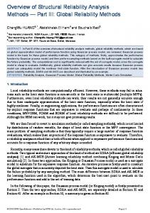
Fig. 1. Operable area of the present formula

k1 =

1 − 3l2 共1 +

l21

−

, l22兲

k2 =

l2 共1 + + 12l22兲 l21

共6c兲

From Eq. 共6b兲, the following condition should be satisfied: ␣4X 艌 共7 + 4␣23X兲/3

共6d兲 ␣23X − ␣4X

plane can Using Eq. 共6d兲, a lower boundary line in the be depicted as shown in Fig. 1, in which the operable area of the present formula is indicated as the shaded region. In Fig. 1, the limit for all distributions expressed as ␣4X = 1 + ␣23X 共Johnson and Kotz 1970兲 is also depicted along with the ␣23X − ␣4X relationship for some commonly used distributions, i.e., the normal, Gumbel, Laplace, and the exponential distribution, which are represented by a single point, the lognormal, the Gamma, the Frechet, and the Weibull distributions—represented by a line—are also depicted. One can see that the operable area of the present formula covers a large area in the ␣23X − ␣4X plane, and the ␣23X − ␣4X relationship for most commonly used distributions is in the operable area of the present formula. This implies that Eq. 共6d兲 is generally operable for common engineering use. When ␣4X = 3 + 4␣23X / 3, one has l1 = ␣3X / 6, k1 = 1 / 共1 + ␣23X / 36兲, and l2 = k2 = 0, then Eq. 共6a兲 can be expressed as 1 xs = k1u − ␣3X共u2 − 1兲 6 when ␣3X is small enough, k1 ⬇ 1, the equation above is simplified as 1 xs = u − ␣3X共u2 − 1兲 6

共7兲

which becomes the first-order Fisher-Cornish expansion. Particularly, if ␣3X = 0 and ␣4X = 3, then l1, l2, k1, and k2 will be obtained as l1 = l2 = k2 = 0 and k1 = 1, and the u-x transformation function will be degenerate as xs = u. From Eq. 共6兲, the x-u transformation is readily obtained as u=−

冑3 2p

冑− q + ⌬ 3

+

冑3 − q + ⌬ l1 冑3 2 − 3k2

共8a兲

where 918 / JOURNAL OF STRUCTURAL ENGINEERING © ASCE / JULY 2007

The four polynomial coefficients—a1, a2, a3, and a4—determined by the proposed formula are illustrated in Fig. 2, compared with those obtained using Fisher-Cornish expansion, Winterstein formula, and the accurate coefficients obtained from momentmatching method 共Fleishman 1978兲. The coefficients are expressed as functions of ␣4X for ␣3X = 0.0, 0.4, 0.8, and 1.2. One can clearly see from Fig. 2 that: 1. The coefficients of Fisher-Cornish expansion have the greatest differences from the accurate coefficients except when the random variable x is nearly a normal random variable. 2. The Winterstein formula markedly improves the FisherCornish expansion and provides good results when ␣3X is small and ␣4X is within a particular range. However, as ␣3X becomes larger, especially when ␣3X is larger than 0.4, the coefficients obtained by the Winterstein formula will have significant differences compared to the accurate ones. 3. The coefficients obtained using the proposed formula are in close agreement with the accurate ones throughout the entire investigation range. As described above, the parameters of an accurate fourthmoment standardization function should make the first four moments of the function Su共u兲 关the right side of Eq. 共6a兲兴 be equal to those of the original random variable 关the left side of Eq. 共6a兲兴. For the given pair value of ␣3X and ␣4X, the polynomial coefficients can be determined by using Eqs. 共6b兲 and 共6c兲 and Eq. 共6a兲 can be thus determined. Since the right side of Eq. 共6a兲 only includes the standard normal variable, the skewness ␣3S and kurtosis ␣4S of Su共u兲 can be easily obtained as ␣3S = 6k21l1 + 8l31 + 72k1k2l1 + 270k22l1

共9a兲

␣4S = 3共k41 + 20k31k2 + 210k21k22 + 1260k1k32 + 3465k42兲 + 12l21共5k21 + 5l21 + 78k1k2 + 375k22兲

共9b兲

Obviously, ␣3S and ␣4S should be equal to ␣3X and ␣4X, respectively, if Su共u兲 is accurate. ␣3S and ␣4S obtained using the present method are depicted in Fig. 3, together with the accurate ones and those obtained using the Fisher-Cornish expansion and Winterstein formula. In Fig. 3, the following two relationships of ␣3X and ␣4X are investigated • Case 1, ␣4X = 2.7+ 1.5␣23X; and • Case 2, ␣4X = 4 + 2␣23X. One can clearly see from Fig. 3 that the relationships between ␣3S and ␣4S obtained by Fisher-Cornish expansion and Winterstein formula differ greatly from the accurate ones, while ␣3S and ␣4S obtained by the proposed formula are in close agreement with the accurate ones. Thus, Eq. 共8兲 is the suggested simple and accurate fourthmoment standardization function. For a random variable, if the first four moments can be obtained, the x-u and u-x transformation can be realized with Eqs. 共8兲 and 共6兲, respectively. Using the proposed method, the structural reliability analysis including the random variables with unknown CDFs/PDFs can be conducted without using the Rosenblatt transformation.

Fig. 2. Comparisons of the determination of polynomial coefficients using four different methods

Reliability Analysis Including Random Variables with Unknown CDFs/PDFs

Fig. 3. Comparison of ␣4S and ␣3S using four different methods

Using the first four central moments of an arbitrary random variable x 共continuous or discontinuous兲 with unknown CDFs/PDFs, a standard normal u can be obtained using Eq. 共8兲, and a random variable x⬘ corresponding to u can be obtained from Eq. 共6兲. Since u is a continuous random variable, x⬘ will also be a continuous random variable. Although x and x⬘ are different random variables, they correspond to the same standard normal random variable, and have the same fourth central moment and the same statistical information source. Therefore, f共x⬘兲 can be considered to be an anticipated PDF of x. Using this PDF, reliability analysis including random variables with unknown CDFs/PDFs will be possible. Because the u-x and x-u transformations are realized directly by using Eqs. 共6兲 and 共8兲, the specific form of f共x⬘兲 is not required in FORM/SORM. Assuming that the random variables with unknown CDFs/PDFs are independent of those that have CDFs/PDFs and are independent of each other as well, from Eqs. JOURNAL OF STRUCTURAL ENGINEERING © ASCE / JULY 2007 / 919

Fig. 4. u-x and x-u transformations for Gumbel random variable

共6兲 and 共8兲, the element of the Jacobian matrix corresponding to a random variable x with an unknown CDF/PDF can be given as Jii =

1 ⳵ui = ⳵xi ␴关k1 + 2l1ui + 3k2u2i 兴

共10兲

For a reliability analysis with all the random variables that have a known CDF/PDF, the analysis can be conducted using the general FORM procedure 共Ang and Tang 1984兲. For a reliability analysis including random variables with unknown CDFs/PDFs, the random variables X can be divided into two groups X = 关X1 , X2兴, where X1 are the random variables that have known CDFs/PDFs, and X2 are those with unknown CDFs/PDFs. For X1, the normal transformation and Jacobian matrix are conducted using the Rosenblatt transformation, and for X2, the normal transformation is conducted using Eq. 共8兲, and the Jacobian matrix are obtained using Eq. 共10兲. Then, the procedure is identical to that of the general FORM, with the exception of the conduction of the normal transformation and the computation of the elements of the Jacobian matrix corresponding to the random variables with unknown CDFs/PDFs. Therefore, the reliability analysis including random variables with unknown CDFs/PDFs using the proposed method requires only minimal extra computational effort, compared to the general FORM procedure. When random variables that have unknown CDFs/PDFs are contained in a performance function with strong nonlinearity, for which a more accurate method such as SORM is required, the proposed method can also be applied. In such a case, the computational procedure is identical to that of general SORM with the exception of the u-x and x-u transformations and the computation of the elements of the Jacobian matrix corresponding to the random variables with unknown CDFs/PDFs.

Numerical Examples u-x and x-u Transformations for Random Variables with Known CDFs/PDFs In evaluating a normal transformation technique, the first concern could be how the relation between non-normal and normal variables is described by the technique. Suppose a random variable x is known to have a PDF, f共x兲, the u-x and x-u transformations can be obtained by using the proposed fourth-moment standardization function or the other aforementioned normal transformation tech920 / JOURNAL OF STRUCTURAL ENGINEERING © ASCE / JULY 2007

niques. Since the Rosenblatt transformation completely preserves the known marginal distribution, that is, F共x兲 = ⌽共u兲, it is used herein as the benchmark in performance evaluation for the other normal transformation techniques. The first example considers a Gumbel random variable that has the following PDF: f共x兲 =

冋 冉 冊 冉 冊册

1 ␣−x ␣−x exp − exp + ␤ ␤ ␤

共11兲

For ␣ = 0.550 and ␤ = 0.780, the mean value, standard deviation, skewness, and kurtosis are obtained as ␮X = 1, ␴X = 1, ␣3X = 1.140, and ␣4X = 5.4, respectively. The variations of the u-x transformation function with respect to u and the variations of the x-u transformation function with respect to xs are shown in Figs. 4共a and b兲, respectively, for the results obtained using the Rosenblatt transformation, the present fourth-moment transformation, the third-moment transformation 共Zhao and Ono 2000兲, the Fisher-Cornish expansion, and the Winterstein formula. Fig. 4 reveals the following: 1. The results of the Fisher-Cornish expansion exhibit the greatest differences from the results obtained by the Rosenblatt transformation, especially when the absolute value of u or xs is large. 2. Since only the information of the first three central moments is used in the third-moment transformation, the method yields significant errors when the absolute value of u or xs is large for this example. 3. The transformation function obtained using the Winterstein formula provides good results when the absolute value of u or xs is small, while when the absolute value of u or xs is large, the results obtained from the Winterstein formula differ greatly from those obtained using the Rosenblatt transformation. 4. The proposed method performs better than the third-moment transformation, the Fisher-Cornish expansion, and the Winterstein formula, and the results of the proposed transformation coincide with those of the Rosenblatt transformation throughout the entire investigation range. The second example considers a lognormal random variable with parameters ␭ = 2.283 and ␨ = 0.198. The mean value, standard deviation, skewness, and kurtosis are obtained as ␮X = 10.0, ␴X = 2.0, ␣3X = 0.608, and ␣4X = 3.664, respectively. The variations of the u-x and x-u transformation are shown in Figs. 5共a and b兲, respectively, for the results obtained using the

Fig. 5. u-x and x-u transformations for lognormal random variable

Rosenblatt transformation, the present fourth-moment transformation, the third-moment transformation, the Fisher-Cornish expansion, and the Winterstein formula. Again, one can clearly see from Fig. 5 that the proposed method performs better than the thirdmoment transformation, the Fisher-Cornish expansion, and the Winterstein formula, and the results of the proposed transformation coincide with those of the Rosenblatt transformation throughout the entire investigation range. Reliability Analysis Including Random Variables with Unknown CDF/PDFs The third example considers the following performance function, which is an elementary reliability model that has several applications: G共X兲 = dR − S

共12兲

where R = resistance having ␮R = 500 and ␴R = 100; S = load with a coefficient of variation of 0.4; and d = modification of R having normal distribution, ␮d = 1 and ␴d = 0.1. The following six cases are investigated under the assumption that R and S follow different probability distributions: • Case 1: R is Gumbel 共Type I-largest兲 and S is Weibull 共Type III-smallest兲;, • Case 2: R is gamma and S is normal; • Case 3: R is lognormal and S is gamma; • Case 4: R is lognormal and S is Gumbel; • Case 5: R is Weibull and S is lognormal; and • Case 6: R is Frechet 共Type II-largest兲 and S is exponential. Because all of the random variables in the performance function have known CDFs/PDFs, the first-order reliability index for the six cases described above can be readily obtained using FORM. In order to investigate the efficiency of the proposed reliability method, including random variables with unknown CDFs/PDFs, the CDF/PDF of random variable R in the six cases is assumed to be unknown, and only its first four moments are known. With the first four moments, the u-x and x-u transformations in FORM can be performed easily using the proposed method, and then the first-order reliability index, including random variables that have unknown CDFs/PDFs, can also be readily obtained. The skewness and kurtosis of R corresponding to cases 1–6 are easily obtained as 1.14 and 5.4, 0.4 and 3.24, 0.608 and 3.664, −0.352 and 3.004, and 2.353 and 16.43, respectively. The firstorder reliability index obtained using the CDF/PDF of R, and

using only the first four moments of R, are depicted in Fig. 6 for mean values of S in the range of 100–500. Fig. 6 reveals that, for all six cases, the results of the first-order reliability index obtained using only the first four moments of R are in agreement with those obtained using the CDF/PDF of R. This is to say that the proposed method is accurate enough to include random variables with unknown CDFs/PDFs. For Case 4, the detailed results obtained while determining the design point using the CDF/PDF of R and using the first four moments of R are listed in Table 1. Table 1 shows that the checking point 共in original and standard normal space兲, the Jacobian, and the first-order reliability index obtained in each iteration using the first four moments of R 共columns 6–9兲 are generally close to those obtained in each iteration using the CDF/PDF of R 共columns 2–5兲. As an application of Example 3, the fourth example considers the following performance function of an H-shaped steel column G共X兲 = AY − C

共13兲

where A = section area; Y = yield stress; and C is the compressive stress. The CDFs of A and Y are unknown. The only information that is known about them is their first four moments 共Ono et al. 1986兲, i.e., ␮A = 71.656 cm2; ␴A = 3.691 cm2; ␣3A = 0.709; ␣4A = 3.692; ␮Y = 3.055t / cm2; ␴Y = 0.364; ␣3Y = 0.512; and ␣4Y = 3.957. C is assumed as a lognormal variable with a mean value of ␮C = 100t and a standard deviation of ␴C = 40t. The skew-

Fig. 6. Comparisons of first-order reliability index with known and unknown CDFs/PDFs JOURNAL OF STRUCTURAL ENGINEERING © ASCE / JULY 2007 / 921

Table 1. Comparisons of FORM Procedure with Known and Unknown CDF/PDFs for Example 3 Using CDF/PDF

Using the first four moments

Checking point Iteration 1

2

5

Checking point

共x兲

共u兲

Jacobian 共dx / du兲

1.000 500.000 200.000 0.916 326.151 284.326 0.947 403.013 381.741

0.000 0.099 0.177 −0.837 −2.058 1.102 −0.528 −0.990 1.881

0.100 99.021 76.492 0.100 64.592 107.917 0.100 79.814 143.638

␤

共x兲

共u兲

Jacobian 共dx / du兲

2.254

1.000 500.000 200.000 0.916 326.142 284.319 0.947 403.132 381.845

0.000 0.099 0.177 −0.836 −2.055 1.102 −0.528 −0.989 1.881

0.100 99.017 76.492 0.100 65.484 107.914 0.100 79.752 143.674

2.219

2.190

ness and kurtosis of C can soon be obtained as ␣3C = 1.264 and ␣4C = 5.969. Although the CDFs of A and Y are unknown, since the first four moments are known, the x-u and u-x transformations can be easily realized using the present method instead of the Rosenblatt transformation, and FORM can be readily conducted with results of ␤FORM = 2.079 and P f = 0.0188. Furthermore, using Eq. 共6兲, the random sampling of A and Y can be easily generated without using their CDFs, and thus, the Monte Carlo simulation 共MCS兲 can be approximately conducted. The probability of failure of this performance function is obtained as P f = 0.0183, and the corresponding reliability index is equal to 2.090 when the number of samples taken is 500,000. The coefficient of variation 共COV兲 of this MCS estimate is 1.035%. One can see that the results obtained by the two methods for this example are almost the same. Application in Point-Fitting SORM The fifth example considers the following performance function; a plastic collapse mechanism of an elastoplastic frame structure with one story and one bay, as shown in Fig. 7 G共X兲 = M 1 + 3M 2 + 2M 3 − 15S1 − 10S2

共14兲

The variables of M i and Si are statistically independent and lognormally distributed, and have means of ␮ M1 = ␮ M2 = ␮ M3 = 500 ft K, ␮S1 = 50 K, and ␮S2 = 100 K, respectively, and COVs of V M1 = V M2 = V M3 = 0.15, VS1 = 0.30, and VS2 = 0.20, respectively. Because all of the random variables in the performance function shown in Eq. 共14兲 have a known CDF/PDF, the reliability index can be readily obtained using FORM/SORM. The FORM reliability index is ␤FORM = 2.851, which corresponds to a failure probability of P f = 2.181⫻ 10−2. Using the MCS method, the reli-

922 / JOURNAL OF STRUCTURAL ENGINEERING © ASCE / JULY 2007

2.254

2.224

2.190

ability index is obtained as ␤MCS = 2.794, and the corresponding probability of failure is equal to 2.603⫻ 10−3. The COV of this MCS estimate is 0.875%. Using the point-fitting SORM 共Zhao and Ono 1999兲, the point-fitted performance function is obtained as G共u兲 = 1219.14 + 73.66u1 + 218.97u2 + 146.75u3 − 151.26u4 − 184.59u5 + 5.20u21 + 14.17u22 + 9.89u23 − 57.05u24 共15兲

− 25.61u25

The average curvature radius is obtained as R = 56.62 and the second-order reliability index 共Zhao et al. 2002兲 is obtained as ␤SORM = 2.816, which corresponds to a failure probability of P f = 2.44⫻ 10−3. In order to investigate the application of the proposed reliability method, including random variables with unknown CDF/PDFs to the point-fitting SORM, the CDFs/PDFs of random variables S1 and S2 are assumed to be unknown, and only the first four moments are known. Using the first four moments, the u-x and x-u transformations can be performed easily using the proposed method, and then the point-fitting SORM, including random variables with unknown CDFs/PDFs, can also be performed easily. The point-fitted performance function is obtained as G⬘共u兲 = 1233.15 + 73.65u1 + 218.97u2 + 146.75u3 − 166.77u4 − 188.82u5 + 5.20u21 + 14.17u22 + 9.89u23 − 52.92u24 共16兲

− 25.26u25

The average curvature radius is given as R = −63.31 and the second-reliability indices is obtained as ␤SORM = 2.817, which corresponds to a failure probability of P f = 2.43⫻ 10−3. One can see that the results obtained using the first four moments of S1 and S2 are very close to those obtained using the CDFs/PDFs of S1 and S2. This is to say that the proposed u-x and x-u transformations are applicable to the point-fitting SORM. The sixth example considers the following strong nonlinear performance function G共x兲 = x41 + x22 − 50

Fig. 7. One-story one-bay frame

␤

共17兲

where x1 and x2 = statistically independent; x1 = lognormal variable with mean value of 5 and COV of 0.2; and x2 = Gumbel variable with mean value of 10 and COV of 1. Because x1 and x2 have a known CDF/PDF, using FORM, SORM, and MCS, the reliability indices can be readily obtained as: ␤FORM = 3.254; ␤SORM = 3.562; and ␤MCS = 3.570 共the COV of

MCS is 3.35%兲. In order to investigate the application of the proposed reliability method, including random variables with unknown CDFs/PDFs to FORM, SORM, and MCS, the CDFs/PDFs of random variables x1 and x2 are assumed to be unknown, and only the first four moments are known. The results are obtained as: ␤FORM = 3.220; ␤SORM = 3.513; and ␤MCS = 3.509 共the COV of MCS is 2.98%兲. Apparently, the results obtained by using the first four moments of x1 and x2 are close to those obtained using the CDFs/PDFs of x1 and x2.

Conclusions 1.

2.

A simple explicit fourth-moment standardization function is proposed. It is found to be accurate enough to include independent random variables with unknown CDFs/PDFs in reliability analysis using FORM/SORM. Since the proposed fourth-moment formula can give a good approximation for the polynomial coefficients using the first four central moments, the present method provides more appropriate u-x and x-u transformation results compared to the third-moment function, Fisher-Cornish expansion, or Winterstein formula.

Acknowledgments The study was partially supported by Grant-in-Aid from the Ministry of ESCST, Japan 共Grant No. 17560501兲. The support is gratefully acknowledged.

Notation The following symbols are used in this paper: a, b, c, and d ⫽ coefficients in the PDF of Pearson system; a1, a2, a3, a4 ⫽ polynomial coefficients used in the third-order polynomial normal transformation; f共X兲 ⫽ joint probability density function of X; G共X兲 ⫽ performance function; h3 , h4 ⫽ Hermite series coefficients 关Eq. 共4兲兴; ˜h , ˜h ,˜k ⫽ Hermite series coefficient 关Eq. 共5兲兴; 3 4 l1 , l2 , k1 , k2 ⫽ coefficients of Eq. 共6兲; P f ⫽ probability of failure; R ⫽ resistance; S ⫽ load; Su共u兲 ⫽ the third polynomial of u; U ⫽ standard normal random variables; u ⫽ standard normal random variable; V ⫽ coefficient of variation; X ⫽ random variables; xs ⫽ random variable corresponding to x with its mean value= 0 and standard deviation = 1; ␣3X ⫽ coefficient of skewness of random variable x; ␣4X ⫽ coefficient of kurtosis of random variable x; ␤FORM ⫽ first-order reliability index; ␤SORM ⫽ second-order reliability index;

␮ ⫽ mean value; ␴ ⫽ standard deviations; and ⌽共x兲 ⫽ standard normal probability distribution with argument x;

References Ang, A. H.-S., and Tang, W. H. 共1984兲. Probability concepts in engineering planning and design, Vol. II: Decision, risk, and reliability, Wiley, New York. Cai, G. Q., and Elishakoff, I. 共1994兲. “Refined second-order reliability analysis.” Struct. Safety, 14共4兲, 267–276. Chen, X., and Tung, Y. K. 共2003兲. “Investigation of polynomial normal transform.” Struct. Safety, 25共4兲, 423–455. Der Kiureghian, A., and De Stefano, M. 共1991兲. “Efficient algorithm for second-order reliability analysis.” J. Eng. Mech., 117共12兲, 2904– 2923. Der Kiureghian, A., Lin, H. Z., and Hwang, S. J. 共1987兲. “Second-order reliability approximations.” J. Eng. Mech., 113共8兲, 1208–1225. Der Kiureghian, A., and Liu, P. L. 共1986兲. “Structural reliability under incomplete probability information.” J. Eng. Mech., 112共1兲, 85–104. Fisher, R. A., and Cornish, E. A. 共1960兲. “The percentile points of distributions having known cumulants.” Technometrics, 2, 209. Fleishman, A. L. 共1978兲. “A method for simulating non-normal distributions.” Psychometrika, 43共4兲, 521–532. Fu, G. 共1994兲. “Variance reduction by truncated multimodal importance sampling.” Struct. Safety, 13共4兲, 267–283. Grigoriu, M. 共1983兲. “Approximate analysis of complex reliability analysis.” Struct. Safety, 1共4兲, 277–288. Hasofer, A. M., and Lind, N. C. 共1974兲. “Exact and invariant second moment code format.” J. Engrg. Mech. Div., 100共1兲, 111–121. Hohenbichler, M., and Rackwitz, R. 共1981兲. “Non-normal dependent vectors in structural safety.” J. Engrg. Mech. Div., 107共6兲, 1227–1238. Hong, H. P. 共1996兲. “Point-estimate moment-based reliability analysis.” Civ. Eng. Syst., 13, 281–294. Hong, H. P., and Lind, N. C. 共1996兲. “Approximation reliability analysis using normal polynomial and simulation results.” Struct. Safety, 18共4兲, 329–339. Johnson, N. L., and Kotz, S. 共1970兲. Continuous univariate distributions—1, Wiley, New York. Liu, P. L., and Der Kiureghian, A. 共1986兲. “Multivariate distribution models with prescribed marginals and covariances.” Probab. Eng. Mech., 1共2兲, 105–116. Liu, Y. W., and Moses, F. 共1994兲. “A sequential response surface method and its application in the reliability analysis of aircraft structural systems.” Struct. Safety, 16共1兲, 39–46. Melchers, R. E. 共1990兲. “Radial importance sampling for structural reliability.” J. Eng. Mech., 116共1兲, 189–203. Nie, J., and Ellingwood, B. R. 共2000兲. “Directional methods for structural reliability analysis.” Struct. Safety, 22共3兲, 233–249. Ono, T., Idota, H., and Kawahara, H. 共1986兲. “A statistical study on resistances of steel columns and beams using higher order moments.” J. Struct. Constr. Eng., 370, 19–37 共in Japanese兲. Pearson, E. S., Johnson, N. L., and Burr, I. W. 共1979兲. “Comparison of the percentage points of distributions with the same first four moments, chosen from eight different systems of frequency curves.” Commun. Stat.-Simul. Comput., B8共3兲, 191–229. Rackwitz, R. 共1976兲. “Practical probabilistic approach to design—Firstorder reliability concepts for design codes.” Bull. d’Information, No. 112, Comite European du Beton, Munich, Germany. Rajashekhar, M. R., and Ellingwood, B. R. 共1993兲. “A new look at the response surface approach for reliability analysis.” Struct. Safety, 12共3兲, 205–220. Ramberg, J., and Schmeiser, B. 共1974兲. “An approximate method for generating asymmetric random variables.” Commun. ACM, 17共2兲, 78–82. Shinozuka, M. 共1983兲. “Basic analysis of structural safety.” J. Struct. JOURNAL OF STRUCTURAL ENGINEERING © ASCE / JULY 2007 / 923

Eng., 109共3兲, 721–740. Stuart, A., and Ord, J. K. 共1987兲. Kendall’s advanced theory of statistics, Charles Griffin and Company Ltd., London, Vol. 1, 210–275. Tichy, M. 共1994兲. “First-order third-moment reliability method.” Struct. Safety, 16共3兲, 189–200. Tung, Y. K. 共1999兲. “Polynomial normal transform in uncertainty analysis.” ICASP 8—Application of probability and statistics, Balkema, The Netherlands, 167–174. Winterstein, S. R. 共1988兲. “Nonlinear vibration models for extremes and fatigue.” J. Eng. Mech., 114共10兲, 1769–1787.

924 / JOURNAL OF STRUCTURAL ENGINEERING © ASCE / JULY 2007

Zhao, Y. G., and Ang, A. H.-S. 共2003兲. “System reliability assessment by method of moments.” J. Struct. Eng., 129共10兲, 1341–1349. Zhao, Y. G., and Ono, T. 共1999兲. “New approximations for SORM: Part II.” J. Eng. Mech., 125共1兲, 86–93. Zhao, Y. G., and Ono, T. 共2000兲. “Third-moment standardization for structural reliability analysis.” J. Struct. Eng., 126共6兲, 724–732. Zhao, Y. G., Ono, T., and Kato, M. 共2002兲. “Second-order third-moment reliability method.” J. Struct. Eng., 128共8兲, 1087–1090. Zong, Z., and Lam, K. Y. 共1998兲. “Estimation of complicated distribution using B-spline functions.” Struct. Safety, 20共4兲, 341–355.