FPGA Architecture for Kriging Image Interpolation - The Science and ...

(IJACSA) International Journal of Advanced Computer Science and Applications, Vol. 4, No. 12, 2013

FPGA Architecture for Kriging Image Interpolation Maciej Wielgosz, Mauritz Panggabean and Leif Arne Rønningen Department of Telematics Norwegian University of Science and Technology (NTNU) N-7491, Trondheim, Norway Abstract—This paper proposes an ultrafast scalable embedded image compression scheme based on discrete cosine transform. It is designed for general network architecture that guarantees maximum end-to-end delay (EED), in particular the Distributed Multimedia Plays (DMP) architecture. DMP is designed to enable people to perform delay-sensitive real-time collaboration from remote places via their own collaboration space (CS). It requires much lower EED to achieve good synchronization than that in existing teleconference systems. A DMP node can drop packets from networked CSs intelligently to guarantee its local delay and degrade visual quality gracefully. The transmitter classifies visual information in an input image into priority ranks. Included in the bitstream as side information, the ranks enable intelligent packet dropping. The receiver reconstructs the image from the remaining packets. Four priority ranks for dropping are provided. Our promising results reveal that, with the proposed compression technique, maximum EED can be guaranteed with graceful degradation of image quality. The given parallel designs for its hardware implementation in FPGA shows its technical feasibility as a module in the DMP architecture.

I.

I NTRODUCTION

Greater interest in green technology and rapid technological advances opens ways to conceive multi-party collaboration from distributed places via tele-immersive environment. Nearnatural quality is achievable by tiling auto-stereoscopic multiview 3D displays and high-end cameras on all the surfaces of such environment. The collaborations will soon include those which are very sensitive to end-to-end delay (EED), such as remote choir-conducting and dancing. The effect of EED is very critical to achieve good synchronization between the collaborating people from different locations. For example, the optimal EED for synchronizing rhythmic clapping hands from different places is 11.5ms [3]. It includes propagation, transmission and all processing delays. Longer EED will produce increasingly severe tempo deceleration while shorter ones yield a modest yet surprising acceleration. Percussion is rhythmically similar to clapping hands. Musicians playing percussion will then require similar EED for both audio and video data while collaborating. The same effect of EED to collaborative dancing is indicated in [22]. Video data is essential to good synchronization between dancers as they depend on visual cues [3]. Thus the greatest demand to meet and guarantee such low EED lies in processing visual information. The Internet today, however, is unable to deliver such guarantee with its best-effort design. One approach for it is to design network nodes with ability to intelligently drop video packets on-the-fly despite changing traffic conditions but also with graceful quality degradation. Video compression by current coding standards is conducted only by the sender.

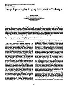
Higher visual quality comes at the expense of more complexity and longer encoding time. Therefore very low EED implies minimizing or even avoiding video coding at the expense of high increase in bit rate. It implies the use of intraframe, object-based and parallel processing. To guarantee both the constant EED and the graceful degradation of visual quality, a novel network architecture namely Distributed Multimedia Plays (DMP) has been proposed [16]. Very demanding situations during collaboration, for example when the input video from the collaboration environment is extremely transient, require simplified approach in processing the data. A simple data representation for parallel image transmission is shown in Fig. 1. N ×N blocks are tiled directly on the pixels of a video frame, yielding N 2 bit streams of pixel values. In DMP objects in an image can be segmented, processed and transmitted independently. The number of pixel streams in a segmented object may vary depending on its visual content. Thus network nodes can drop pixel streams after entropy coding to instantly reduce the bit rate according to immediate traffic conditions.

Fig. 1. The tiling of 3 × 3 blocks (N = 3) over an image of 9 × 9 pixels, yielding N 2 = 9 streams of pixels (left); the dropping of streams number 3, 4 and 8 (right). Each pixel of dropped streams denoted by × will be optimally interpolated from the remaining ones at the receiver.

The time for data reduction by network nodes must also be minimized. This affects how the entropy coding must be designed later. The dropped pixels will be estimated by applying optimal interpolation in the sense of mean square error to the received bit streams at the receiver. Searching for such interpolation leads us to Kriging, a technique wellknown and widely used in geostatistics. Kriging works better by using window mechanism, hence called windowed kriging interpolation. It was proposed and used to interpolate luma and chroma data in natural images with positive results [12][13]. The collaboration system on the DMP algorithm must work fast due to the very low EED. Practically it means that the processing routines are to be implemented in hardware. In this work we focus on field-programmable gate array

193 | P a g e www.ijacsa.thesai.org

(IJACSA) International Journal of Advanced Computer Science and Applications, Vol. 4, No. 12, 2013

(FPGA) implementation. To the best of our knowledge, there is no reliable reported information on the feasibility of FPGA architecture for Kriging image interpolation. This work is motivated to fill that void. Some of the calculation routines in the proposed architecture are reused. Moreover some highly exhaustive computations are skipped whenever possible. The paper is structured as follows. Section II presents an in-depth analysis of the Kriging algorithm that leads to the proposed FPGA architecture. The computational complexity and the resource consumption of the architecture are discussed in Section III. Section IV finally concludes the paper with the summary and some ideas for future work. II.

A NALYSIS OF THE K RIGING A LGORITHM AND THE P ROPOSED A RCHITECTURE

The computational cost of some parts of the Kriging algorithm is O(n4 ) where n is the size in pixels of the square image interpolated. The strong data dependencies in the algorithm make parallelization a challenge. Some of the inherently sequential stages in the algorithm are best performed on general purpose processor (GPP) rather than on FPGA.

Fig. 2.

The image reconstruction scheme in DMP.

B. Step 2: Constructing the Variogram Matrix A variogram provides the information on the contribution of a given point to that being reconstructed [7]. It is a function of a distance vector between the points h as γ(h) = 21 E[(z(si +h)−z(si ))2 ] where z(si ) are observations in two different locations separated by h. A variogram is obtained from an experimental semivariance as a result of its fitting to one of variogram models [7], [11]. Experimental semivariance for each distance h in an interpolated image frame may be obtained as γ(h) =

Implementations of the Kriging algorithm on different computational platforms of GPP or graphics processing unit (GPU) have been reported such as in [6][4][8][17]. The speedup factors are promising and span from eight [6][4], twelve [17] and up to 120 [8]. The latter is achieved on GPU by means of compute unified device architecture (CUDA). The architecture for OK presented in this paper aims to decrease the overall latency in FPGAs. Therefore direct use of the aforementioned speedup benchmarks is not adequate for DMP. The goal of most of these implementations is to reach high data-processing throughput rather than low system latency. This is understandable as most of the papers focus on geology and geostatistics [6][4][8][17] instead of image processing. Nevertheless there are some work that cover the latter in [10][5][14] although they do not address FPGA implementation. Ordinary kriging (OK) is employed in this work to interpolate the dropped pixels in an output image. ML605 platform from Xilinx [18] is chosen for system deployment and estimates. The analysis consists of three computational steps of the OK algorithm [7]. Step 1 is to find points in an image which contribute to building an output picture. Step 2 is to construct the variogram matrix. The last step is to compute the weights and interpolate the missing points. A. Step 1: Finding Points as Basis for Interpolation The step for the windowed Kriging interpolation [11] is not very difficult since all the input points to be considered are included in the well-established frame of interest of D×D pixels. The optimal size of D is a subject of research and will be provided later in this paper. A DMP access-node reconstructs an image out of the received packets according to the employed dropping scheme [1]. The number of dropped packets varies depending on the network traffic. Image data in pixels are gradually delivered to the Kriging interpolation module (KIM) which is responsible for the image reconstruction. An overview of the process is depicted in Fig. 2.

N (h) X 1 E[(z(si + h) − z(si ))2 ] 2N (h) i=1

(1)

where N (h) denotes the number of sample pairs separated by h [7]. There are five stages to compute the variogram: 1)

Determining the squares of the distances between all the points in the area of interest constituted by the D × D window Sorting the distances Accumulating the sorted values Building an experimental variogram Fitting the variogram to an appropriate model.

2) 3) 4) 5)

The computational complexity of the first stage can be shown as D2 (D2 − 1)/2 ≈ O(D4 ). The operations in this stage involve both subtraction and multiplication of each pair of the D × D pixels. Multipliers and adders in Stage 1 are connected in a pipeline fashion to the other modules, as illustrated in Fig. 3. The overall number of different inter-pixel distances within a picture, N (D), is given by (2 + D − 2)! 2(D − 2)! D(D − 1) (D − 1)(D + 2) = + (D − 1) = 2 2 where D is the length of an image frame edge in pixels. N (D) is plotted against D in Fig. 4. N (D) = ( D + 12 ) + (D − 1) =

A separate hardware module can be dedicated to each processing stream, as encircled in black in Fig. 3, leading to N (D) streams. The number of pixels processed by a single stream in such a scheme is expressed by total number of pixels in a picture overall number of distances between pixels   D2 (D2 − 1)/2 = (D − 1)(D + 2)/2   2 D (D + 1) = ≈ D2 . D+2

k=

194 | P a g e www.ijacsa.thesai.org

(IJACSA) International Journal of Advanced Computer Science and Applications, Vol. 4, No. 12, 2013

achieve the final precision of 8 bits, some guard bits are used in the middle processing stages (see Fig. 3). However to simplify the analysis, this parameter is set to 0, i.e. no guard bits. Unfortunately the pixel pairs are not evenly distributed across the streams. For example, from 2D(D − 1) pairs of neighboring pixels, two are of the maximum distance, i.e. the diagonal of an image frame. Therefore the architecture (without MUX) illustrated in Fig. 3 is not optimal in terms of data distribution. Some of the streams will finish their tasks earlier and remain idle while the others are still being processed. Load balancing procedure may be implemented as finite state machine (FSM) to provide equal distribution of pixels across the streams. This procedure would require driving MUXs that feed the accumulators with data according to the computed semivariance. However, the delay introduced by the MUXs is large, due to their sizes and resource consumption.

Fig. 3.

The proposed architecture of the variogram calculation module.

Fig. 4.

The number of different distances as a function of D.

Note that this approach leads to large memory consumption since N (D) of k KB Block RAMs (BRAMs) or distributed RAM memory blocks are required. It is because a separate memory port is needed for data fetching and reading. Sorting can be performed during the data fetching or by means of a set of (N (D) to 1) multiplexers (MUXs). The pipeline architecture of the variogram calculation unit presented in Fig. 3 features all the processing stages of Step 2. There are 4[(D − 1)(D + 2)/2] units in a variogramcalculation module with an approximately 10 clock cycles (CLKs) + MUX pipeline latency. Here the variogram-fitting module is not taken into account. It is assumed that a multiplier consumes 3 CLK while an adder and an accumulator take 1 CLK. The pipeline delay also depends on the data width. To

An interesting alternative would be time-multiplexing of variogram computations coupled with an accumulator-result summation. Instead of implementing a set of MUXs, Eq. (1) may be multiplexed in time, reusing the streams in Fig. 3 multiple times during computations. The decision regarding the number of parallel streams should consider the expected size of the input image. Fig. 5 plots the variogram computation time for one stream against D. The estimate assumes that the FPGA is clocked at 100 MHz. The remaining part of the paper also adopts that assumption. As mentioned above, computation time depends on the degree of parallelism. In the case of variogram calculation stage, it is strictly related to the number of processing streams employed. Fig. 6 exhibits this relationship, as a function of the number of concurrently working module for D that equals 256, 128 and 64 pixels.

Fig. 5.

Computation time of a single stream against D.

The throughput of the external data bus is a key factor in estimating the system performance. There are two communication buses employed in DMP: PCIe and 10Gb Ethernet. The transfer speed of the latter is 2 or 1.25 GB/s. PCIe bus is used for local data transfer between the camera devices and the processing boards. The 10Gb Ethernet provides the inter-node communication [15]. Fig. 7 reflects the expected throughput of the two interfaces for different values of D. Raw transfer that includes the overhead of the protocols is considered here for simplicity. The worst case in Fig. 7 occurs when only one pixel is missing and must be interpolated from the input data. In real situation it will not occur since the smallest amount of data being dropped is 1/N 2 of all the image pixels. The

195 | P a g e www.ijacsa.thesai.org

(IJACSA) International Journal of Advanced Computer Science and Applications, Vol. 4, No. 12, 2013

resources at 64 streams drops to approximately 11% and the computation time remains below 1ms, as shown in Fig. 6. The analysis presented in this section does not cover variogram fitting procedure due to its sequential nature. Moreover the other blocks in Fig. 3 absorb many resources. Thus the computation of variogram matrix is assumed to be made offline and uploaded to the FPGA before the computations start. This section is intended to show that implementing Step 2 on FPGA is feasible. It may be attempted later with high probability. It would be especially beneficial if some of the other modules presented later in the paper, e.g. the linear solver, could be reused for this purpose. It is saved for future research, along with studying the impact of using fixed variogam on the quality of the image interpolation. By fixed variograms we mean using the same variogram matrix for different images, instead of generating a different one for each new incoming frame. Fig. 6. The impact of the number of concurrently employed streams on the computation time.

C. Step 3: Computing the Coefficients and Interpolation This step is performed directly after Step 2 and implemented as a separate hardware module. It is again useful to skip the experimental variogram fitting. Therefore it is assumed here that the variogram matrix is computed offline and uploaded to FPGA internal memory. This does not exclude the possibility of incorporating the generation of the variogram matrix into the system later. Step 3 features two operations that are implemented as separate hardware modules. The first is the construction of the semivariogram matrix. The second is to solve the linear equation to compute the λ coefficients.

Fig. 7.

A variogram matrix can be built by gradually filling it up with data derived from the model equations. The following exponential model is the most suitable for image interpolation   (2) f (h) = c 1 − e−3h/a

Data transfer/computational time against D.

number of dropped pixels varies from 1/N 2 to (N 2 − 1)/N 2 , either fully or partially (cf. Fig. 1). Fig. 7 also depicts how the growth of an image size affects both the data transfer and computation time as shown by the dotted green line. One can see that the computation time, rather than the data transfer, is the constraint. Consequently it is possible to generate a variogram for quite large images given enough parallel streams. Here we focus on 256×256 images. A single stream absorbs roughly 270 look-up tables (LUTs), 252 flip-flops (FFs) and one BRAM [19]. Thus a single Virtex-6 XC6VLX240T chip can accommodate 150,720/270 ≈ 558 streams if the timemultiplexing is chosen, i.e. no resource is reserved for implementing MUXs. Accordingly, a module comprising 256 streams capable of handling computations of a 256×256 image consumes roughly 46% of all the FPGA resources. It generates results in approximately 10 CLK or 0.1 µs. The stream switching tasks in the time multiplexing takes additional time, but completing the computations under 1µs is feasible. It is possible to reduce resource utilization by reducing the number of parallel streams at the expense of higher multiplexing effort. For instance, the consumption of

where h, a, c are the parameters computed in Step 2 or uploaded to FPGA memory [16]. The model can be implemented as hardware module that consists of a exp() unit, a subtractor and multipliers, as pictured in Fig. 8. Parameters h, a, c and ln(c) are computed offline, e.g. on a GPP. Since there are only four parameters, it is possible to store a few sets of them in the internal memory and use a pointer to the selected one. The selection could be made based on the properties of each incoming image. To reduce resource consumption, the last multiplier in Fig. 8 (b) can be eliminated by computing ln(c) as shown in Fig. 8 (a). If the variogram matrix is implemented as a LUT memory, the number of the entries equals N (D) as shown in Fig. 4. Thus it is important to take into account the available memory resources. For example, 256×256 pixel image occupies roughly 1% of the internal BRAM memory resources of the Xilinx Virtex-6 XC6VLX240T. Depending on the available FPGA resources, one can adopt a strategy by either calculating the variogram values using Eq. (2) or storing a computed variogram matrix in the internal memory. However, regardless of how the variogram matrix is generated, it is passed on to the linear solver.

196 | P a g e www.ijacsa.thesai.org

(IJACSA) International Journal of Advanced Computer Science and Applications, Vol. 4, No. 12, 2013

is to be stored in the memory and used. The data throughput of the module can be efficiently doubled. The example of Cholesky transformation for a 3×3 matrix is as follows: " # " #" # a11 a12 a13 l11 0 0 l11 l12 l13 a21 a22 a23 = l21 l22 0 0 l22 l23 . a31 a32 a33 l31 l32 l33 0 0 l33 Multiplying the matrices in Eq. (5) and solving the set of six equations by forward-substitution lead to the formula that defines an algorithm for a general case as ajk =

k X

ljs · lks

for 1 ≤ k ≤ j ≤ n

(6)

s=1

where j, k, s are matrix indices. Eq. (6) can be defined as ! k−1 X 1 ajk − ljs · lks for j > k ljk = akk s=1

lkk

v u k−1 u X 2 lks = takk −

(7)

s=1

Fig. 8.

Two block diagrams of the f (h) module.

1) The linear equation solver: The goal of the Kriging procedure is to interpolate the missing image pixels at the DMP receiver. Thus, based on the variogram matrix generated in the previous step of the algorithm, it is essential to compute the λi coefficients for every missing point p separately as p=

n X

λi w(xi )

(3)

i=1

where λi and w(xi ) are the coefficient vectors and the values at the known points, respectively [11]. The equation for computing λi in matrix formulation is given by      λi 1 λ λp = (4) µ 1 1T 0 where λi is the variogram matrix and λp is the semivariance vector of the points being interpolated. Since Eq. (4) is solved for all the missing points using the same variogram matrix, one can compute the inverse matrix or use one of the well-known factorization schemes to simplify the calculations, such as QR, LU or Cholesky decompositions. Although the computational complexity of these transformations is O(n3 ), the cost in hardware implementation is different. Neither QR nor LU takes the symmetry of the matrix directly into account. It leads us to use Cholesky decomposition. FPGA implementation of Cholesky decomposition has been studied and reported in many papers such as [9][20][2]. 2) Cholesky decomposition: Cholesky factorization can be performed for symmetric positive definite matrices and this is the case for the variogram matrix. The decomposition scheme is given by A = L LT (5)

The square root occurrence in Eq. (7) is a drawback from hardware implementation perspective. The computation order exhibits data inter-dependencies as shown by   1  2 3   . . 5 . 2 4 ... 2n − 1 The disadvantages can be overcome by incorporating a third matrix D as A = L D LT . (8) The example of 3×3 Cholesky transformation can be computed by setting # " D1 0 0 0 D2 0 . D= 0 0 D3 General expressions for Eq. (8) with respect to l become ! k−1 X 1 ajk − ljs · lks · dk for j > k (9) ljk = akk s=1 dk = akk −

k−1 X

2 · dk lks

(10)

s=1

where j, k, s are indices of the matrices. A naive implementation of Eq. (9) is straightforward for relatively small matrices. However, when the size of the matrix grows, logic consumption and complexity of the module rise significantly. Thus an alternative approach has been adopted based on the concept introduced in [21]. Given a matrix

where A and L are the input matrix and the lower triangular matrix, respectively. It is worth noting that only one matrix L

An−1 = Ln−1 Dn−1 ATn−1 ,

(11)

197 | P a g e www.ijacsa.thesai.org

(IJACSA) International Journal of Advanced Computer Science and Applications, Vol. 4, No. 12, 2013

a new matrix  An =  =  =

can be expressed as  An−1 x xT p  Ln−1 0 Dn−1 0 zT 1 LTn−1 Ln−1 Dn−1 LTn−1 zTn−1 Dn−1



LTn−1 z 0 1  Ln−1 Dn−1 z . zzT Dn−1 + dn 0 dn



Equaling the relevant elements of the matrices yields the following set of equations x = Ln−1 Dn−1 z

(12)

p = zzT Dn−1 + dn

(13)

dn = p −

n−1 X

dk z2k

(14)

k=1

where Eq. (12) can be presented as Ln−1 Dn−1 z = x

(15)

Ln−1 y = x

(16)

Dn−1 z = y

(17)

Fig. 9.

A pipeline architecture for Cholesky decomposition.

The solution of Eq. (15) is derived from Eqs. (16) and (17) via substitution. 3) Architecture of the Cholesky decomposition module: The architecture of the proposed Cholesky factorization module is explained by using the 4×4 matrix example used to generate the 5×5 matrix. The structure of the module shown in Figs. 9 and 10 is based on Eqs. (12-17) which are exemplified as follows.       1 x1 d1 0 0 0 z1  l21 1   0 d2 0 0   z2   x2  =  l  0 0 d 1 0   z3   x3  31 l32 3 x4 l41 l42 l43 1 z4 0 0 0 d4 

1

 l21  l 31 l41

1 l32 l42

1 l43

d1  0  0 0

0 d2 0 0

0 0 d3 0



   x1 y1   y2   x2   y  =  x  3 3 x4 y4 1 

   0 z1 0   z2   = 0   z3   d4 z4

 y1 y2  y3  y4 Fig. 10.

We conceptualize two architectures of the hardware module. The first is a strongly pipeline architecture depicted in Fig. 9. It can be utilized for small matrices, but the implementation for larger matrices can be quite problematic. It may serve as an alternative for the second architecture which is more scalable, cf. Fig. 10. The first architecture delivers results every clock cycle but it works properly only for a dedicated and limited matrix size. Multiple uses of the structure would not be straightforward if there is a need to compute 6×6 matrices in contrast to the second architecture which can process matrices of arbitrary sizes. Nevertheless the implementation of the scalable architecture imposes a challenge. The control unit must be designed such that the idle states are minimized. The

A scalable architecture for Cholesky decomposition.

TABLE I.

T HE EXECUTION STEPS OF 5 × 5 MATRIX CALCULATION MODULE .

Step 1

Step 2

Step 3

y1 = x1 y2 = x2 − l21 y1 y3 = x3 − l31 y1 y4 = x4 − l41 y1

y3 = x3step1 − l32 y2 y4 = y4step1 − l42 y2

y4 = x4step2 − l43 y3

processing phases should overlap according to Table I and Eqs. (12-17). Fig. 11 shows the structure of the linear solvers

198 | P a g e www.ijacsa.thesai.org

(IJACSA) International Journal of Advanced Computer Science and Applications, Vol. 4, No. 12, 2013

The number of CLK cycles required for a single iteration of Eq. (10) as denoted by NCLK is expressed as NCLK =

1 + (Dp − 1) Dp = 2Np 2Np

where Np is the number of parallel processing units. The worst case or the longest computation time occurs when only one processing unit in Fig. 10 is implemented. The number of all the CLK cycles required to calculate a complete matrix A, denoted as NCLK complete , is proportional to the size of the variogram matrix formed for a given image Dp . It is given by NCLK

Fig. 11.

The internal structure of the C0, C1, C2 building blocks.

complete

= Dp NCLK =

D2 . 2Np fp

Approximately 33,000 clock cycles are needed in the worst case when computing a 256×256 LDLT matrix as shown in Fig. 12. It is when both the decimation factor fd and the number of parallel units equal 1. Assuming that the FPGA is clocked at 100 MHz, it takes roughly 330µs to perform the computation.

in the two architectures. The algorithm defined by Eqs. (12-14) is based on a gradual decomposition. It is conducted in a row-wise fashion by iteratively solving triangular linear equations starting with the top-left element of the matrix A. As shown in Fig. 10, one triangular linear solver can be used for the whole procedure and subsequently to compute the λ coefficients via Eq. (4). Unlike the calculation of the missing points which is performed multiple times, a variogram matrix is computed just once. The Cholesky decomposition module is one of those to be implemented on FPGA such as the network units, e.g. router, framer composers and decomposers, quality shaping blocks, and the PCIe components [15]. Due to the scalability of the architecture, it is possible to trade the size of the linear solver for accommodating the other modules in FPGA. III.

C OMPUTATIONAL C OMPLEXITY AND FPGA R ESOURCE C ONSUMPTION

A. Computational Complexity There is a tight relationship between the number of the known pixels and the size of the matrix A in Eq. (11). The less pixels are known, i.e. the more pixels to be interpolated, the smaller A becomes, which means less computations involved in its decomposition. On the other hand, a low number of original pixels present in the final picture means a large number of them are to be interpolated. This results in multiple instances of Eqs. (3) and (4) to be solved as the following arguments. The number of points Dp to be used for calculating the matrix A in Eq. (10) is given by s D2 D =√ (18) Dp = fd fd where D is the size of the original matrix (the length of the original image edge in pixels) and fd denotes the decimation factor (the number of the dropped points).

Fig. 12. The number of CLK cycles essential to compute a complete an LDLT matrix as a function of the decimation factor or the number of computational cores as given by Eq. (18).

The number of the missing points Dm is given by   1 Dm = D2 − Dp2 = D2 1 − . fd Interpolating each of the missing points requires performing the following series of matrix operations to generate the λ coefficients: An λ = γp (19) Ln Dn LTn λ = γp

(20)

Ln y = γp

(21)

Dn LTn γ = y

(22)

Dn z = y

(23)

LTn

(24)

γ = z.

The computation of Eqs. (22) and (23) can be performed in one step due to the properties of the linear solver. Twice more operations are needed for calculating a missing point than for generating an L D LT matrix.

199 | P a g e www.ijacsa.thesai.org

(IJACSA) International Journal of Advanced Computer Science and Applications, Vol. 4, No. 12, 2013

The number of CLK cycles required for a single iteration of λ vector generation, denoted by NCLK λ , is given by NCLK

λ

= 2 NCLK =

Dp . Np

Computing NCLK complete point , which denotes the number of CLK cycles required to compute all the missing points, follows the equation below: NCLK

complete point

= Dm NCLK = D3

λ

fd − 1 3/2

! .

Np fd

The computational complexity of the routine for calculating the missing points is O(D3 ). Vector p in Eq. (3) can be calculated in parallel to solve the linear equations for the missing points. The λ coefficients being generated can be used right away in Eq. (4). It means that, as the λ coefficients are generated for a given point, its value is also computed. This operation can be implemented as a multiplier accumulator block or a single DSP48E. Therefore it is not accounted for in computing NCLK complete point .

DSP48E1 and 832 18Kb BRAM memories [19]. Thus a single Virtex-6 XC6VLX240T can accommodate 150720/217 = 694 C2 blocks, the basic building cores of the linear solver. The limitation here is the number of LUT memories. The estimate does not account for available DSP48 blocks. TABLE II.

R ESOURCE CONSUMPTION OF THE LINEAR SOLVER BUILDING BLOCKS IN F IGS . 9 AND 10.

Module

#LUT

#FF

#DSP slices

#BRAM

C0 C0 (DSP) C1 C2 C2 (DSP)

123 0 332 217 70

110 0 343 233 91

0 1 0 0 1

0 0 0 0 0

If all 694 C2 modules are exhausted to compute the 256 × 256 missing points, the total processing time would drop to 50ms/694 ≈ 0, 072ms. Unfortunately only a part of all the FPGA resources can be devoted to KIM unless there is a separate FPGA dedicated only for its implementation. Fig. 14 presents a block diagram of an exemplary KIM which is capable of processing three windows in parallel [11].

For D = 256 pixels and a single computational core, the number of clock cycles needed to compute all the missing points reaches 5×106 CLK cycles (see Fig. 13). The computational time in this case is roughly 50ms, assuming that the FPGA is clocked at 100 MHz. It is far beyond the system latency limit. This is the worst-case assumption, which means that all the 256×256 points are to be interpolated. In practice the case when the smallest fd is N 2 as in Fig. 1 never occurs.

Fig. 14.

A block diagram of a Kriging interpolation module.

The module works as follows. The Frame Splitting unit divides the image in window size chunks and sends them to the Window Formatting blocks. The Window Formatting unit builds a matrix of the known pixels locations and the set of vectors of unknown points. These will subsequently be fed into the Variogram Matrix Constructing module. In most cases it is just a LUT memory. The module generates a variogram matrix and passes the results to the λ Computing and Interpolation Module. As the architecture depicted in Fig. 14 is scalable, an arbitrary number of processing streams may be chosen. The optimal performance is achieved when the number of the processing streams is equal to the number of windows [11]. Fig. 13. The number of CLK cycles essential for interpolating the missing points in an input image.

B. Resource Consumption The estimated FPGA resource consumption in a Xilinx Virtex-6 XC6VLX240T for the building blocks in Figs. 9 and 10 is presented in Table II. A Xilinx ML-605 board equipped with a Virtex-6 XC6VLX240T is the chosen FPGA platform for the Kriging module implementation. The FPGA contains 241,152 logic cells, 150,720 LUTs, 301,440 FFs, 768

Let us assume that a single processing stream is used to process 256 × 256 images. It absorbs 25% of all the resources of Virtex-6 XC6VLX240T. Note here that 173 units of C2 are used, cf. Fig. 11. In that case the generation of the A = L D LT matrix takes 330µs/173 ≈ 1.9µs and computing all the missing points lasts 4 × 0, 072ms = 0, 288ms. The overall execution time is expected to be roughly 0,3ms in such a case. The assumption of 25% logic utilization is reasonable because it leaves space for implementing the remaining modules, e.g. PCIe, DDR3 memory controller, DMA and Microblaze.

200 | P a g e www.ijacsa.thesai.org

(IJACSA) International Journal of Advanced Computer Science and Applications, Vol. 4, No. 12, 2013

IV.

C ONCLUSION AND FUTURE DIRECTION

The Kriging interpolation module (KIM) is a part of the quality shaping scheme which is considered as one of key components of the future networked collaboration system. Controlled dropping of packets leads to graceful quality degradation. This is achieved provided an effective interpolation mechanism is implemented for very demanding situations. Therefore FPGA realization of kriging is critical and requires special effort to meet a very strict EED of 11ms. A scalable KIM architecture is proposed and its implementation feasibility is analyzed with respect to the DMP system. It poses several challenges to be addressed as future work, such as the implementation of the variogram fitting routine and the impact of using fixed variogram matrix on the quality of the interpolation. The modularity of the proposed architecture makes its future modification or extension straightforward. The latency introduced by the module is less than 1ms for a 256 × 256 image. R EFERENCES [1]

[2]

[3] [4]

[5]

[6] [7]

[8]

[9]

[10]

[11]

[12]

[13]

[14]

[15]

H. Berge, M. Panggabean, and L.A. Rønningen, ”Modelling videoquality shaping with interpolation and frame-drop patterns,” in Proc. 23rd Norsk informatikkonferanse (NIK), 2010, pp. 132–143. D. Besiris, V. Tsagaris, N. Fragoulis, and C. Theoharatos, ”An FPGAbased hardware implementation of configurable pixel-level color image fusion,” IEEE Trans. Geoscience and Remote Sensing, vol. 50, no. 2, pp. 362–373, 2005. C. Chafe, M. Gurevich, G. Leslie, and S. Tyan, ”Effect of time delay on ensemble accuracy,” in Proc. Int’l Symp. Musical Acoustics, 2004. T. Cheng, D. Li, and Q. Wang, ”On parallelizing universal kriging interpolation based on OpenMP,” in Proc. 9th Int’l Symp. Distributed Computing and Applications to Business Engineering and Science (DCABES), 2010, pp. 36–39. E. Decenciere, C. de Fouquet, and F. Meyer, ”Applications of kriging to image sequence coding,” Signal Processing: Image Communications, vol. 13, no. 3, pp. 227–249, 1998. F. He, J. Fang, and W. Zou, ”An effective method for interpolation,” in Proc. 19th Int’l Conf. Geoinformatics, 2011, pp.1–6. T. Hengl, A Practical Guide to Geostatistical Mapping, Joint Research Centre Institute for Environment and Sustainability, European Commission, 2009. M. Li and L. Dong, ”Visualization three-dimensional geological modeling using CUDA,” in Proc. 6th Int’l Conf. Image and Graphics (ICIG), 2011, pp. 852–857.

[16]

[17]

[18] [19] [20]

[21]

[22]

O. Maslennikow, P. Ratuszniak, and A. Sergyienko, ”Implementation of Cholesky LLT-decomposition algorithm in FPGA-based rational fraction parallel processor,” in Proc. 14th Int’l Conf. Mixed Design of Integrated Circuits and Systems, 2007, pp. 287–292. A. Panagiotopoulou and V. Anastassopoulos, ”Super-resolution image reconstruction employing Kriging interpolation technique,” in Proc. 14th Int’l Workshop on Systems, Signals and Image Processing (IWSSIP), 2008, pp.114–147. ¨ Tamer, and L.A. Rønningen, ”Parallel image transM. Panggabean, O. mission and compression using windowed kriging interpolation,” in Proc. 10th IEEE Symp. Signal Processing and Information Technology (ISSPIT), 2010, pp. 315–320. M. Panggabean and L.A. Rønningen, ”Chroma interpolation using windowed kriging for color-image compression-by-network with guaranteed delay,” in Proc. 17th Int’l Conf. Digital Signal Processing (DSP), 2011, pp.1–6. M. Panggabean and L.A. Rønningen, ”Parameterization of windowed kriging for compression-by-network of natural images,” in Proc. 7th Int’l Symp. Image and Signal Processing and Analysis (ISPA), 2011, pp. 373–378. J. Ruiz-Alzola, C. Alberola-Lopez, and C.F. Westin, ”Kriging Filters for Multidimensional Signal Processing,” Signal Processing, vol. 85, no. 2, pp. 413–439, 2005. L.A. Rønningen, The DMP System and Physical Architecture, Technical Report, Department of Telematics, Norwegian University of Science and Technology, 2007. ¨ Tamer, ”Toward futuristic L.A. Rønningen, M. Panggabean, and O. near-natural collaborations on Distributed Multimedia Plays architecture,” in Proc. 10th IEEE Symp. Signal Processing and Information Technology (ISSPIT), 2010, pp.102–107. J. Strzelczyk, S. Porzycka, and A. Lesniak, ”Analysis of ground deformations based on parallel geostatistical computations of PSInSAR data,” in Proc. 17th Int’l Conf. Geoinformatics, 2009, pp.1–6. Xilinx, http://www.xilinx.com/products/boards-and-kits/EK-V6ML605-G.htm, (2012). Xilinx, http://www.xilinx.com/support/documentation/data sheets/ds150. pdf, (2012). Ch. Xuezheng, K. Benkrid, and J. Thompson, ”Rapid prototyping of an improved Cholesky decomposition based MIMO detector on FPGAs,” in Proc. NASA/ESA Conf. Adaptive Hardware and Systems, 2009, pp.369–375. D. Yang, G. Peterson, and H. Li, ”High performance reconfigurable computing for Cholesky decomposition,” in Proc. Symp. Application Accelerators in High Performance Computing (SAAHPC), 2009. Z. Yang, B. Yu, W. Wu, K. Nahrstedt, R. Diankov, and R. Bajscy, ”A study of collaborative dancing in tele-immersive environments,” in Proc. 8th Int’l Symp. Multimedia, 2006, pp. 177–184.

201 | P a g e www.ijacsa.thesai.org