FPGA-friendly Code Compression for Horizontal Microcoded Custom IPs

FPGA-friendly Code Compression for Horizontal Microcoded Custom IPs Bita Gorjiara and Daniel Gajski Center for Embedded Computer Systems University of California, Irvine

{bgorjiar, gajski}@cecs.uci.edu ABSTRACT

1. INTRODUCTION

Shrinking time-to-market and high demand for productivity has driven traditional hardware designers to use design methodologies that start from high-level languages. However, meeting timing constraints of automatically generated IPs is often a challenging and time-consuming task that must be repeated every time the specification is modified. To address this issue, a new generation of IP-design technologies that is capable of generating custom datapaths as well as programming an existing one is developed. These technologies are often based on Horizontal Microcoded Architectures. Large code size is a well-know problem in HMAs, and is referred to as “code bloating” problem.

Shrinking time-to-market and high demand for productivity has driven traditional hardware designers to use design methodologies that start from high-level languages. However, meeting timing constraints of automatically generated IPs is often a challenging and time-consuming task for designers. Moreover, slight changes in the high-level specification require re-running the behavioral synthesis tools, producing a new datapath, and redoing the process of meeting timing constraints. To avoid repeating timing-closure phase, a new generation of custom-IP design technology that is capable of both generating custom datapaths as well as re-programming existing ones (without further modifications) is developed. In these technologies, first a custom datapath is generated for an application, and then the datapath is synthesized and laid out properly to meet timing and physical constraints. The final step is to compile the program on the generated datapath. If the application is changed after synthesis, it is simply recompiled on the existing datapath. This feature significantly improves the productivity of the designer by avoiding repetition of timing closure phase. Examples of such technology include ARM OptimoDE [1], [2], NISC [4], [5], [6], and TIPI [7]. These techniques are targeted for statically-scheduled Horizontal Microcoded Architectures (HMA) [8].

In this paper, we study the code size of one of the new HMAbased technologies called NISC. We show that NISC code size can be several times larger than a typical RISC processor, and we propose several low-overhead dictionary-based code compression techniques to reduce the code size. Our compression algorithm leverages the knowledge of “don’t care” values in the control words to better compress the content of dictionary memories. Our experiments show that by selecting proper memory architectures the code size of NISC can be reduced by 70% (i.e. 3.3 times) at cost of only 9% performance degradation. We also show that some code compression techniques may increase number of utilized block RAMs in FPGA-based implementations. To address this issue, we propose combining dictionaries and implementing them using embedded dual-port memories.

Categories and Subject Descriptors C.3 [Special-Purpose and Application-based Systems]: Microprocessor/microcomputer applications.

General Terms Algorithms, Design, Performance, Experimentation.

Keywords Microcoded Architectures, No-Instruction-Set Computer, Memory optimization, Dictionary-based compression, FPGA. Permission to make digital or hard copies of all or part of this work for personal or classroom use is granted without fee provided that copies are not made or distributed for profit or commercial advantage and that copies bear this notice and the full citation on the first page. To copy otherwise, or republish, to post on servers or to redistribute to lists, requires prior specific permission and/or a fee. FPGA’07, February 18–20, 2007, Monterey, California, USA. Copyright 2007 ACM 978-1-59593-600-4/07/0002...$5.00.

A microcode is a set of bits that controls the units of datapath for one cycle. In statically scheduled HMAs, the compiler compiles the program directly to microcode without instruction abstraction. HMAs can potentially have better performance, lower power, and lower area than conventional RISC processors. This is due to replacing the costly hardware schedulers with off-line compiler algorithms. As a result, highly parallel architectures can be designed as HMA without any concern about the complexity of controller and hardware scheduler. Despite all these benefits, HMAs suffer from code size problem, known as “code bloating”. This paper studies the code size of a new HMA-based design methodology, called NISC, and compares it with that of traditional RISC processors. We observed that although NISC IPs outperform RISC processors by five times on average, their code sizes are about four times larger than those of RISC. In this paper, we propose low-overhead, yet effective, code compression techniques for NISC IPs targeted for FPGAs. Our compression approach is based on dictionary-based compression algorithms. In our approach each microcode (or control word) is partitioned to two or more slices and dictionaries of unique slices are constructed. The compressed code contains the addresses of slices in the dictionaries. Our

experiments show that optimum number of dictionaries varies for different application sizes. Our approach has very low performance overhead (i.e. 9% on average) and can compress NISC binaries by 3.3 times. Such significant savings makes the code size of NISC only 16% (on average) worse than that of traditional RISC processors. We also show that some of the proposed code compression techniques, despite decreasing the code size, increase number of utilized block RAMs in FPGAbased implementations. We address this issue by combining dictionaries and implementing them using embedded dual-port memories. This paper is organized as follows: Section 2 presents an overview of related works. Section 3 presents a motivational example that compares the performance and code size of NISC with RISC. Section 4 presents our code compression techniques followed by experimental results in Section 5. Section 6 concludes the paper.

2. RELATED WORKS In the past, a large body of code-size-reduction techniques for processors has been proposed. The techniques can be categorized in three groups: (1) Compiler optimizations: techniques such as register renaming, inter-procedural optimization, and procedural abstraction can be implemented in compiler to reduce the code size [12], [13], [14], [15], [16]. These techniques can be applied to microcoded architectures as well, and they are out of scope of this paper. (2) Instruction set: instruction-set abstraction is often used to reduce the code size of processors. In RISC processors, designers define 32-bit or 16-bit [17] [18] instructions to encode wide control words. At runtime, the instructions are decoded back to the control words using a hardware decoder. The software development tools must also support and utilize the instructions. However designing instruction-set is a very complex and time-consuming task for a typical IP designer; because compiler, assembler, linker and instruction decoder must be re-designed to handle the custom instructions. Furthermore, the instruction decoder imposes unnecessary hardware overhead in custom IPs. Therefore, it is desirable to avoid instruction-set abstraction. (3) Code compression: in these techniques, the executable program is compressed offline and decompressed on-the-fly during execution. Code compressions affect only memory structure without changing compiler or processor architecture. Most proposed code-compression techniques are based on dictionary-based compression algorithms. In [19], a dictionarybased compression technique, known as CCRP, was proposed in which instruction cache is modified to run compressed programs. In this approach, unique instructions in the program are stored in a dictionary, where the location of the instructions is determined by Huffman coding. Most frequent instructions in the program are placed in low addresses of the dictionary and are coded with less number of bits. Due to Huffman coding, the compressed instructions have variable sizes. At runtime, the compressed codes are fetched from main memory, decompressed and put in the instruction cache. In this approach cache misses are problematic because missed

instructions in the cache do not reside at the same address in main memory. CCRP uses a Line Address Table (LAT) to map missed instruction cache addresses to main memory addresses where the compressed code is located. IBM CodePack [20], [21], [22] is another compression technique that has the same memory structure as of CCRP. In CodePack, each instruction is partitioned to two halves and two dictionary memories are used to store the unique patterns of each half. CodePack also uses Huffman encoding to gain better compression ratio. Both CCRP and CodePack are complex and have high decompression delay. Therefore, they rely on using cache to hide the decompression latency. However, in most custom IPs, cache imposes an unnecessary hardware overhead and is often avoided. As a result, these compression techniques are not easily applicable. In [23], the authors extend the twodictionary architecture (i.e. CodePack) by rearranging the instruction bits to balance the size of the two dictionaries. Also, in [24] and [25], the authors extend the concept of dictionary-based compression to sequence of instructions. In these approaches, unique sequences of instructions are identified and stored in a dictionary memory. In the executable code, these sequences are replaced by the corresponding codewords. These approaches also result in variable code size and need cache for hiding the latency. Furthermore, they need additional controller hardware to run the sequence of instructions. The proposed code-compression techniques increase the hardware complexity significantly by requiring complex cache structures. Therefore they are not suitable for custom IPs. In this paper, we study the efficiency of multi-dictionary compression techniques on code size of applications compiled on NISC. We use one to four dictionaries in our compression approaches, and show that optimum number of dictionaries varies for different application sizes. To reduce the delay of decompression, we use a fixed size coding style, which can be implemented even without cache. Our dictionary compression algorithm leverages the knowledge of “don’t care” values in the control words to better compress the content of dictionaries. We also show that some code compression techniques, despite decreasing the code size, increase number of utilized block RAMs in FPGA-based implementations.

3. MOTIVATIONAL EXAMPLE To study the code size of HMA-based architectures we choose NISC technology, since we had access to its toolset. NISC technology is HMA-based and it relies on a sophisticated compiler [5] to compile a program described in a high-level language to binary that directly drives the control signals of components in the datapath. The values of control signals generated for each cycle are called a Control Word (CW). The CWs are stored in Control Memory (CMem) in programmable IPs, while they are synthesized to lookup-table logic in hardwired dedicated IPs. In NISC, the area is relatively small because of elimination of instruction decoder and hardware scheduler. However, the code size is very large compared to RISC processors.

Table 2- Comparing GN with MicroBlaze

RF

MicroBlaze

CW

PC

CMem

Benchmarks AG

COMP

ALU

MUL

DMem

DIV

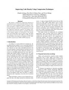
Figure 1- Block diagram of GN architecture. To compare NISC with RISC, we designed datapath shown in Figure 1, called GN, and synthesized it on Xilinx FPGA using NISC tools [4]. The GN architecture has a register file (RF), a comparator (COMP), an ALU, a multiplier (MUL), and a divider (DIV), where some of the units are pipelined. Since NISC tools generate synthesizable code for Xilinx FPGA, we choose Xilinx MicroBlaze for comparing RISC and NISC on the same platform. We configured MicroBlaze to include a divider core, and synthesized both processors on a Xilinx Virtex4 (90nm) FPGA package using ISE 8.1. Table 1 shows the area and clock frequency of the processors. Both processors could run at about 100MHz, while the area of GN is smaller than MicroBlaze.

#cycles

adpcm_coder 256748693 adpcm_decoder 322766405 CRC32 209436647 dijkstra 25927532 sha 183030479 Mp3 2668445 Average

code size (KB) 1.956 1.364 1.264 1.928 3.156 44.62

GN vs. MicroBlaze code size speedup code size (KB) (x) ratio 6.960 3.45 5.10 5.075 5.12 2.59 2.567 9.56 2.03 9.614 2.66 4.99 14.123 9.49 4.47 216.659 2.97 4.86 5.54 4.01

GN #cycles 74321930 63082673 21901993 9764682 19282976 897452

4. OUR CODE COMPRESSION APPROACH The dictionary based compression techniques rely on the fact that same binary patterns (BP) appear many times in the program. Figure 2 shows how these techniques typically work. If a program has N instructions and each instruction is n bits, then N×n bits must be stored in the memory. If the number of distinct BPs is M and m=log2M is much smaller than n, then a dictionary based technique can compress the code down to N×m+M×n bits in the memory instead of N×n. However, this compression costs one extra memory access during CW fetch.

Table 1- Area and clock frequency of MicroBlaze and GN Processors MicroBlaze GN

Clock freq.(MHz) 105 100

Area (gates) 39574 32632

We compiled and ran a set of benchmarks including dijkstra, sha, adpcm_coder, adpcm_decoder and CRC32 from MiBench (the free version of EEMBC embedded benchmarks available at [10]), and a fixed-point Mp3 decoder (more than 10,000 lines of C code available at [11]). For each benchmarks, to get the accurate execution cycle count, we generated and simulated RTL Verilog code of the design. Table 2 shows the number of cycles and code size of each benchmark on the two processors. MiBench provides a small and a large input for the benchmarks. The reported cycle numbers are for simulating the small input of MiBench benchmarks. For simulating the Mp3 decoder, we used the scope1.mp3 (44.1KHz, 96kbit/s, stereo) available at [11], and ran the simulation to process 1 frame of the Mp3 file. For these experiments, we set the compiler optimizations to the maximum level to achieve the best performance with both NISC and MicroBlaze. The code size of MicroBlaze (third column) is the size of instruction section (.text) of the .elf file generated by the compiler. The sixth column shows speedup of GN compared to MicroBlaze. The seventh column shows the ratio of GN code size to that of MicroBlaze. On average GN runs 5.54 times faster than MicroBlaze, while its code size is four times larger. The large code size increases the size of control memory, in programmable IPs, and the area of control logic, in dedicated IPs. The goal of our code optimization technique is to reduce the code size of NISC processors while maintaining the performance benefits.

Figure 2-Dictionary-based code compression To reduce the code size, we construct a dictionary of unique Control Words (CWs) and, in the executable binary, replace control words by the corresponding dictionary line addresses. Figure 3 shows a one-dictionary code compression approach. The memory structure consists of a code lookup table (CodeLUT) and a dictionary. The Program Counter (PC) contains the address of CodeLUT and is used to fetch the next code word. The code word is then used to fetch the corresponding control word from dictionary. CodeLUT Dictionary

lookup

lookup

Figure 3- One-dictionary code compression (opt1) Suppose that Figure 4 shows the control words of a sample program. Each control word has 16 bits and the program has nine control words. Therefore, the code size of the program is 144 bits (16×9). Figure 5 shows the compressed

implementation of Figure 4, where the dictionary contains five unique control words and the CodeLUT contains the corresponding address of the CWs. To address the dictionary three bits is needed, thus the code words are three-bit wide. After compression the total memory size is reduced to 107 (i.e. 3×9+16×5). 0 1 1 1 1 0 0 1 0 1

1 0 0 0 0 0 0 0 0 0

2 0 0 0 0 1 1 0 1 0

3 1 0 1 0 0 0 1 0 1

4 0 1 0 1 1 1 0 1 0

5 1 1 1 1 0 0 1 0 1

6 1 1 1 1 1 1 1 1 1

7 0 1 0 1 0 0 0 0 0

8 0 0 1 0 1 1 0 1 1

9 0 0 1 0 0 0 0 0 1

10 11 12 13 14 15 1 0 1 0 1 0 1 0 1 0 1 0 1 0 1 0 1 0 1 0 1 0 1 0 0 0 1 1 1 1 0 1 0 1 1 0 1 0 1 0 1 0 0 0 1 1 1 1 1 0 1 0 1 0

Figure 4- Control words of a sample program 000 001 010 000 011 100 001 011 010

0 1 1 1 0 0

1 0 0 0 0 0

2 0 0 0 1 1

3 1 0 1 0 0

4 0 1 0 1 1

5 1 1 1 0 0

6 1 1 1 1 1

7 0 1 0 0 0

8 0 0 1 1 1

9 0 0 1 0 0

10 1 1 1 0 0

11 0 0 0 0 1

12 1 1 1 1 0

13 0 0 0 1 1

14 1 1 1 1 1

Figure 7, Figure 8, and Figure 9 show two-, three- and fourdictionary code compression approaches called opt2, opt3, and opt4, respectively. Since all the dictionaries are accessed in parallel, more dictionaries do not affect the performance penalty. In NISC the control words are relatively wide (50 bits or more depending on the architecture features). Since the size of performance-critical applications implemented using custom IPs is usually small, the number of unique control words is usually small as well. Therefore, the dictionaries can be addressed with relatively few bits. Consequently, the width of code words is far smaller than the width of control words. This property makes it possible to reduce code size using multiple dictionaries without requiring Huffman encoding. Without Huffman encoding, the width of all code words becomes the same and the decoding becomes easier.

15 0 0 0 1 0

Figure 5- Single-dictionary compression on control words of Figure 4 00 01 00 00 10 10 01 10 00

00 00 01 00 10 11 00 10 01

0 1 1 0

1 0 0 0

2 0 0 1

3 1 0 0

4 0 1 1

5 1 1 0

6 1 1 1

7 0 1 0

8 0 1 1 1

9 0 1 0 0

10 11 12 13 14 15 1 0 1 0 1 0 1 0 1 0 1 0 0 0 1 1 1 1 0 1 0 1 1 0

Figure 7- Two-dictionary code compression (opt2)

Figure 6- two-dictionary compression on control words of Figure 4 Since CWs can be very wide with many unique patterns, the dictionary may have many entries. To increase the chances of finding matching patterns, we partition the CWs to smaller slices and construct multiple dictionaries. Usually the total code size of the partitioned dictionaries is much smaller than that of a single big dictionary. However, corresponding to each dictionary, a code field must be added to code words. Figure 6 shows the two-dictionary implementation of the example control words shown in Figure 4. The top dictionary contains the unique patterns of the least-significant half of the control words, while the bottom dictionary has those of the mostsignificant halves. Note that number of unique control word slices in each half is less than total number of unique control words. The code words have two fields to address the two dictionaries. Since each dictionary has four or less entries, the code word fields are only two bits. Using two-dictionary implementation the code size is reduced to 92 bits (i.e. 4×9+8×3+8×4). As number of dictionaries increases, the number of CodeLUT fields increases. As a result, at some point, the size increase of CodeLUT cancels out the gain of having more dictionaries.

Figure 8- Three-dictionary code compression (opt3)

Figure 9- Four-dictionary code compression (opt4)

4.1 Reducing number of block RAMs The CodeLUT and dictionaries may be implemented using hardwired lookup tables or programmable memories (RAM), depending on the design re-programmability goals. If all are implemented using RAM, the datapath is completely reprogrammable. However, if dictionaries are implemented

using hardwired logic, and CodeLUT is implemented using RAM, the reprogramming is limited to applications that contain the hardwired CWs.

Figure 10- Two-dictionary code compression using a dualport memory (opt2DP)

respectively. Note that, the merged dictionary contents may have more entries than each individual dictionary. However, the size of the merged dictionary is less than the total size of the two dictionaries, because redundant entries can be removed after merging the contents. Since merging dictionaries increase the depth of the dictionary unit, the width of code words may increase as well. As a result, the total code size may remain the same as before, but number of utilized block RAMs decreases. Figure 13 shows the dictionary content and CodeLUT of the dual-port implementation of Figure 6. The seven entries of the two dictionaries in Figure 6 are compacted to four unique entries in Figure 13. The code words are also updated to refer to the correct bit patterns. Compared to Figure 6 that requires three block RAMs, Figure 13 requires only two RAMs. Also, the code size is reduced to 68 bits (i.e. 4×9+8×4). 11 00 10 00 11 01 11 00 00 10 00 11 10 00 00 10 11 01

0 1 1 1

0 1 0 0

1 1 0 0

0 0 0 1

1 1 1 0

0 0 1 1

1 1 1 1

0 0 1 0

Figure 13- dual-port memory implementation of Figure 6

4.2 Smart resolution of “don’t care” bits Figure 11- Three-dictionary code compression using a dual-port memory (opt3DP)

Figure 12- Four-dictionary code compression using two dual-port memories (opt4DP) In today’s FPGAs, tens or even hundreds of compact and fast memory blocks exist. Each block has a predefined size: for example, in Xilinx Virtex4 FPGA, each block RAM is 18Kbits. Although our code compression techniques reduce the code size, they tend to increase number of memory (or LUT) units, thus occupying more under-utilized block RAMs. For very small programs that only occupy one block RAM, the dictionary-based compression approach is not suitable, because it increases number of utilized block RAMs to two or more. To reduce number of utilized RAMs in larger programs that occupy more than one RAMs, we propose to integrate every two available dictionaries into one dual-port memory. Since in FPGAs, one block RAM can be configured as single-port or dual port, integrating dictionaries can help in reducing number of utilized RAMs. Figure 10, Figure 11, and Figure 12 show the dual-port implementation of opt2, opt3, and opt4,

In NISC, each control word contains values of control signals in the datapath. At each cycles, some of the control signals in the datapath may have “don’t care” values. This means that either ‘0’ or ‘1’ can be assigned to those control signals without affecting the correctness of the program. For example, if a 4-input Mux unit is not used in a given cycle, its selection signal can be assigned ‘00’, ‘01’, ‘10’ or ‘11’. NISC compiler maintains the information of “don’t care” values and marks them by ‘X’ in the output binary. Some of the control signals such as register-file write enable cannot be ‘X’, because if ‘X’ gets resolved to ‘1’, an incorrect data is written to the RF. Control signals such as register-file read and write addresses, Mux selection signal, and ALU operation signal can be ‘X’ when the units are not used. Figure 14 shows an example of NISC control words. 1 0 X 1 0

0 X 0 X 0

X X 0 0 X

X 1 1 X 1

1 1 X 1 1

1 0 1 X 0

X 0 0 0 X

X 0 1 X 0

X 1 0 0 1

1 X X 1 0

1 0 X 1 0

0 X 0 X 0

X X 0 0 0

0 1 0 X 1

1 1 X 1 1

Figure 14- Example of control words generated by NISC compiler To build a dictionary for CWs of Figure 14, one may replace ‘X’ values by ‘0’ and then extract the unique patterns. In that case, the dictionary (shown in Figure 15) will have four entries, because only the second and the last vectors match. However, if the ‘X’ values are smartly resolved, then the dictionary will have only two entries shown in Figure 16. The ‘X’ values can be resolved so that the first, third, and fourth vectors in Figure 14 are mapped to the first entry of Figure 16, and the other two vectors are mapped to the second entry of Figure 16.

1 0 0 1

0 0 0 0

0 0 0 0

0 1 1 0

1 1 0 1

1 0 1 0

0 0 0 0

0 0 1 0

0 1 0 0

1 0 0 1

1 0 0 1

0 0 0 0

0 0 0 0

0 1 0 0

1 1 0 1

Figure 15- Dictionary content for CWs of Figure 14 (‘X’ are replace by ‘0’) 1 0 0 1 1 1 0 1 0 1 1 1 0 0 1 0 0 0 1 1 0 0 0 1 0 0 0 0 1 1

Figure 16- Dictionary content for CWs of Figure 14 (using smart ‘X’ resolution) The problem that must be solved is to resolve ‘X’ values in CWs so that the total number of unique patterns is minimized. To solve this problem, we convert it to graph coloring [27] problem. For a given list of bit-vectors, we construct a graph G(V, E), where the vertices in V are the bit-vectors, and the edges in E show the conflict between the vectors. Two bitvectors v1 and v2 do NOT have conflict if they can be merged to a single bit vector: ∀i∈{1,…, N}, v1[i]=v2[i] OR v1[i]=’X’ OR v2[i]=’X’ Where, N is the number of bits in a bit-vector. The edges in E are defined between the vectors that have conflict with each other: E = {(v1, v2) | v1 has conflict with v2} The algorithm must partition the vertices (or vectors) to subcategories so that there is no edge (i.e. conflict) between any two vertices in the same category while minimizing the total number of categories. This is exactly the graph coloring problem where each category is represented by a distinct color [27]. Solving the graph coloring problem optimally is NP-hard [26]. But there are many well-known heuristics that generate efficient results in polynomial time. After coloring the graph, corresponding to each color a new vector is generated and all the same-color vectors are merged into that vector. The new vectors are used to fill the dictionary. Figure 17 shows our dictionary compression algorithm in more details. First a conflict graph is constructed from the given set of bit-vectors V. Then, using the graph coloring algorithm, a color is assigned to each vector and the set of generated colors (i.e. C) is returned back to the algorithm. For each color in the set, a new combined bit-vector cv is created and all of its bits are initialized by ‘X’. Then, all the same-color vectors are merged into their corresponding cv, and the remaining ‘X’ bits are replaced by ‘0’. The final compact bit vectors (i.e. CV) are used to fill the content of a dictionary.

5. EXPERIMENTAL RESULTS We implemented all the compression techniques, opt1 (Figure 3), opt2 (Figure 7), opt3 (Figure 8), opt4 (Figure 9), opt2DP (Figure 10), opt3DP (Figure 11), and opt4DP (Figure 12). We used the benchmarks of Section 3 in these experiments as well. In Section 5.1, compression techniques are compared in terms of their Code Compression Ratio. In Section 5.2, compression techniques are compared in terms of number of utilized block RAMs in a fully programmable RAM-based implementation. Finally, in Section 5.3 the performance penalty of the techniques is presented.

Compress (V, N) //Inputs: //V: the list of vectors //N: the bit width of the vectors //output: CV, the list of compact vectors. G = ConstructConflictGraph(V); C = Color(G); // C is the set of colors for each color c in C // create a new vector that contains only ‘X’ cv = new BitVector('X', N ); for each v in V if (color of v is c) //merging the two vectors for i=1 to N if(v[i] != 'X') cv[i] = v[i]; for each v in CV replace the remaining 'X' in v with '0' CV.Add(cv); return CV;

Figure 17- Our dictionary compression algorithm

5.1 Code-size comparison Table 3 shows the code size of the benchmarks running on NISC with different code compressions. The second column shows the baseline code size of NISC with no code compression (No-opt). As number of dictionaries increases (columns 3, 4, 5, and 6), the code size (i.e. the total size of dictionaries and CodeLUT) of all the benchmark decrease up to certain points (the highlighted values) and then increases again. These are the points where the increase in CodeLUT size cancels out the benefit of having more dictionaries. As shown in the table, the minimum point for each benchmark is different and depends on the baseline size of the benchmarks. For CRC32, which is the smallest benchmark, four dictionaries (i.e. opt4) achieve the minimum code size. For medium size benchmarks (adpcm_coder, adpcm_decoder, dijkstra, and sha), the minimum code size is achieved with three dictionaries (i.e. opt3). For MP3, which is significantly larger than others, the two-dictionary compression (i.e. opt2) is the best. Nevertheless, on average, the code size is reduced by 3.3 times comparing the best compressed code sizes to the baseline (No-opt column). The last row in the table shows the Code Compression Ratio (CCR) a metric commonly used to evaluate a compression algorithm. CCR is the ratio between the compressed size and the original size, and smaller CCR numbers show a better compression. On average for all these benchmarks, the threedictionary compression (i.e. opt3) outperforms the others with CCR of 0.3. Note that without Huffman encoding, multiple dictionaries can easily outperform the single-dictionary compression. Furthermore, these experiments highlight that number of dictionaries must be selected based on the size of the target applications, to achieve the minimum code size. In these experiments, using dual-port memories does not improve code size compared to single-port memory implementation.

Table 3- Code size of benchmarks with different code compressions Memory size (Kbytes) No-opt

adpcm_coder adpcm_decoder CRC32 dijkstra sha Mp3 average CCR

6.96 5.08 2.57 9.61 14.12 216.66 1.00

opt1

opt2

opt3

opt4

opt2DP opt3DP opt4DP

3.77 2.44 2.19 2.19 2.53 2.30 2.49 3.24 1.98 1.59 1.68 2.04 1.76 1.80 1.72 1.04 0.85 0.80 1.06 0.88 0.85 4.32 2.71 2.52 2.68 2.86 2.78 2.93 6.75 4.45 4.12 4.14 4.69 4.63 4.88 82.00 63.08 67.66 76.05 68.72 73.43 81.84 0.53 0.34 0.30 0.31 0.35 0.33 0.34

Table 4- Code size of GN-opt vs. MicroBlaze Memory size (Kbytes) GN-opt vs. MBlaze adpcm_coder adpcm_decoder CRC32 dijkstra sha Mp3 average

MBlaze

GN-opt

code ratio

1.956 1.364 1.264 1.928 3.156 44.62

2.19 1.59 0.80 2.52 4.12 63.08

1.12 1.16 0.63 1.31 1.41 1.31 1.16

By selecting the fittest code compression technique, the code size of NISC becomes very close to that of MicroBlaze. Table 4 compares the code size of the MicroBlaze (second columns) with the best compressed code size of benchmarks (i.e. third column; GN-opt). The fourth column shows the ratio of GNopt code size vs. that of MicroBlaze. For adpcm_coder and adpcm_decoder, NISC code size is only 12% and 16% worse than that of MicroBlaze. For CRC32, NISC code size is even 40% less than MicroBlaze. However, for dijkstra, sha, and MP3, the code size is still 30%-40% more than MicroBlaze. On average, the code size of fittest NISC is only 16% more than the code size of MicroBlaze.

5.2 Block RAM utilization comparison Although opt2, opt3, and opt4 significantly reduce the code size in the lookup-table-based implementation, in a fully programmable RAM-based implementation, they may even increase number of used block RAMs compared to the baseline. In FPGAs, logical memories are implemented using one or more block RAMs depending on their width, depth, and available primitives [28]. Table 5 shows the number of utilized 18Kbit block RAMs in different implementations on Xilinx Virtex4SX35. This package contains hundreds of block RAMs. In MicroBlaze implementation (second column), most of the benchmarks need only one block RAM for their code, except for sha and Mp3, which need two and 21 blocks, respectively. These numbers are significantly higher for NISC (third column), because the CWs are wide, and block RAM primitives do not support wide words. In terms of block RAM utilization, NISC requires on average five times more blocks than MicroBlaze. As expected, most of the compression techniques increase the number of block RAMs for the smaller applications (i.e. adpcm_coder, adpcm_decoder, and CRC32). However, for medium and large applications (i.e. dijkstra, sha, and Mp3), the compression techniques reduce number of block RAMs. Using dual-port memories (i.e. opt2DP, opt3DP, and opt4DP) reduces number of utilized block RAMs compared to single-port memories. The minimum number of blocks is achieved using opt2DP for adpcm_coder, adpcm_decoder, CRC32, dijkstra, and sha. For Mp3 decoder, however, the minimum is achieved

using opt2. That is due to a significant size increase in CodeLUT of MP3 when using dual-port dictionaries. Note that although opt3 is the best compression technique in terms of code size (as shown in Table 3), it wastes many block RAMs in FPGA implementation. In terms of number of utilized block RAMs, opt2DP is more efficient than others. These experiments show that the code compression techniques must take the underlying physical memory structure into account in order to really reduce number of used block RAMs in FPGAs. Otherwise, it may even increase number of used RAMs. Also, note that for partially programmable IPs where dictionaries are implemented with hardwired logic, NISC with compression can easily achieve the same block RAM utilization as of MicroBlaze. Furthermore, these results may vary for different block RAM sizes and available primitives. Table 5- Number of utilized 18Kbit block RAMs. Memory size (number of 18Kbit Block RAMs) MBlaze No-opt opt1 opt2 opt3 opt4 opt2DP opt3DP opt4DP adpcm_coder 1 4 5 6 6 7 3 4 4 adpcm_decoder 1 3 4 5 5 6 2 3 3 CRC32 1 3 4 5 5 6 2 3 3 dijkstra 1 6 5 6 7 9 3 5 5 sha 2 11 5 6 9 11 4 5 5 Mp3 21 117 67 34 38 38 36 42 43

5.3 Performance penalty of code compression All the proposed optimizations have the same performance penalty. They increase the number of fetch pipeline stages by one, which increases the branch delay by one cycle. We described the new architectures for NISC tools in GNR format [29] and ran the compiler to generate the executable code. We modified the tools to generate RTL code for new memory structure and simulated the generated code using Modelsim simulator. In Table 6, the second column shows number of cycles that each benchmark takes to finish after applying optimizations. The third column shows the performance overhead of memory optimization in terms of the slowdown percentage compared to the baseline GN. These numbers are computed using number of cycles with and without code compression (see Table 2 column fourth as well). The performance penalty depends on the average basic block length and that how well the compiler can fill the extra branch delay slot. On average, the performance is degraded only 9.12%. The fifth column compares the speed of optimized GN with that of MicroBlaze processor. The optimized GN is on average 5.21 times faster than MicroBlaze. This shows that the memory optimizations had little effect on the performance of GN. Table 6- Comparing performance of GN-opt with that of GN and MicroBlaze Benchmarks adpcm_coder adpcm_decoder CRC32 dijkstra sha Mp3 Average

GN-opt (with compression) #cycles 84251684 66504319 26008604 10631310 18371827 927307

GN-opt. vs. GN slowdown (%) 13.36 5.42 18.75 8.88 3.33 4.96 9.12

GN-opt. vs. MicroBlaze speedup (x) 3.05 4.85 8.05 2.44 9.96 2.88 5.21

6. CONCLUSION In this paper, we study the code size of NISC IPs and compare it with that of traditional RISC processors. We observed that although NISC IPs outperform RISC processors by five times on average, their code sizes are about four times larger than that of RISC. We study the use of different variations of dictionary-based code compression techniques on NISC binary. Our experiments show that optimum number of dictionaries varies depending on the application size. By selecting proper code compression technique the code size of NISC can be reduced by 70% (i.e. 3.3x) at cost of only 9% performance degradation. Furthermore, we show that some code compression techniques, despite reducing the code size, may increase number of utilized block RAMs in FPGA-based implementations. To address this issue, we propose to merge the content of every two dictionaries into a single dual-port memory. Using this technique, block-RAM utilization is reduced up to 60%.

7. REFERENCES [1] M. Byatt, “Data plane processing with configurable architectures”, ARM white paper, 2003. [2] N. Clark, H. Zhong, K. Fan, S. Mahlke, K. Flautner, K. Van Nieuwenhove, “OptimoDE: Programmable Accelerator Engines Through Retargetable Customization”, Hot Chips, 2004. [3] S. Bashford, U. Bieker, B. Harking, R. Leupers, P. Marwedel, A. Neumann, D. Voggenauer, “The MIMOLA Language - Version 4.1. Technical Report.” Computer Science Dpt., University of Dortmund, 1994. [4] http://www.cecs.uci.edu/~nisc [5] M. Reshadi, D. Gajski, “A cycle-accurate compilation algorithm for custom pipelined datapaths”, In Proc. CODES+ISSS, 2005. [6] M. Reshadi, B. Gorjiara, D. Gajski, “Utilizing Horizontal and Vertical Parallelism Using a No-Instruction-Set Compiler and Custom Datapaths”, International Conference on Computer Design (ICCD), pages 69-76, 2005. [7] S. J Weber and K. Keutzer, “Using minimal minterms to represent programmability”, In Proc. CODES+ISSS, 2005. [8] A. Agrawala, T. Rauscher, Foundations of Microprogramming: Architecture, Software, and Applications, Academic Press, ISBN: 0120451506, 1976. [9] R. Lysecky and F. Vahid, “A study of the speedups and competitiveness of FPGA soft processor cores using dynamic hardware/software partitioning”, Proc. DATE 2005, 2005. [10] MiBench benchmark: http://www.eecs.umich.edu/mibench/ [11] MAD: MPEG Audio Decoder: http://www.underbit.com/products/mad/ [12] K. D. Cooper and N. McIntosh, “Enhanced code compression for embedded RISC processors”, Proc. Conf. on Programming Languages Design and Implementation, 1999.

[13] D. Kirovski, J. Kin, and W. H. Mangione-Smith, “Procedure based program compression”, Proc. 30th Ann. International Symp. on Microarchitecture, 1997. [14] S. K. Debray, W. Evans, R. Muth, and B. De Sutter, “Compiler techniques for code compaction,” ACM Transaction on Programming Languages and Systems, 2000. [15] A. Halambi, A. Shrivastava, P. Biswas, N. Dutt, and A. Nicolau, “An efficient compiler technique for code size reduction using reduced bit-width ISAs,” Proc. Design Automation and Test in Europe, 2002. [16] S. Y. Liao, S. Devadas, and K. Keutzer, “Code density optimization for embedded DSP processors using data compression techniques,” Proc. Chapel Hill Conf. Adv. Res.VLSI, pp. 393–399, 1995. [17] S. Segars, K. Clarke, and L. Goudge, “Embedded control problems, Thumb, and the ARM7TDMI,” IEEE Micro, vol. 15, no. 5, pp. 22–30, Oct. 1995. [18] R. Grehan, “16-bit: The good, the bad, your options,” Embedded Systems Programming, 1997 [Online]. Available: http://www.embedded.com/1999/9908/9908sr.htm [19] A. Wolfe and A. Chanin, “Executing compressed programs on an embedded RISC architecture,” Proc. International Symposium on Microarchitecture, 1992. [20] IBM, CodePack PowerPC code Compression Utility User’s Manual Version 3.0, IBM, 1998. [21] T.M. Kemp, R.K. Montoye, D.J. Auerback, J.D. Harper, J.D. Palmer, “A decompression core for PowerPC”, IBM Syst. J. 42,6(November), 1998. [22] C. Lefurgy, E. Piccininni, T. Mudge, “Evaluation of a high performance code compression method”, In Proc. International Symposium on Microarchitecture, 1999. [23] G. Pechanek, S. Larin, T. Conte, “Any-size instruction abbreviation technique for embedded DSPs”, ASIC/SoC Conference, 2002. [24] M. Corliss, E. Lewis, and A. Roth. “DISE: a programmable macro engine for customizing applications.” Proceedings of the International Symposium on Computer Architecture (ISCA), 2003. [25] C. Fraser. “An instruction for direct interpretation of LZ77compressed programs.” Technical Report MSR-TR-2002-90, Microsoft Research, Microsoft Corporation, 2002. [26] M. Garey and D. Johnson, Computers and Intractability: A Guide to the Theory of NP-Completeness. W.H. Freeman. ISBN 0-7167-1045-5. [27] T. Jensen, B. Toft, Graph coloring problems. WileyInterscience, New York, 1995, ISBN 0-471-02865-7. [28] Xilinx Product Specification, “Block memory generator”, version 1.1, 2006. [29] B. Gorjiara, M. Reshadi, P. Chandraiah, D. Gajski, “Generic netlist representation for system and PE level design exploration,” International Conference on Hardware/Software Codesign and System Synthesis (CODES+ISSS), 2006.