Alignment Process Feature Estimation and Learning (APFEL): For the last ap- proach we use machine learning techniques to gain an presumably optimal align-.
Framework for Ontology Alignment and Mapping Marc Ehrig, Steffen Staab and York Sure Abstract Semantic alignment between ontologies is a necessary precondition to establish interoperability between agents or services using different individual ontologies. This cannot be done manually beyond a certain complexity and size of ontologies. The core contribution in this article is the Framework for Ontology Alignment and Mapping (FOAM). With FOAM we address requirements from an application-based perspective such as high quality results, efficiency, high degree of automation with optional user-interaction, flexibility with respect to use cases, and easy adjusting and parameterizing. FOAM consists of a general alignment process based on the ontology-encoded semantics, different instantiations of the process focusing on various aspects of ontology alignment, and finally the concrete implementation as a powerful but easy to use Open Source tool. The evaluation results show that the different instantiations individually outperform existing approaches. However, best results can be gained when combining them. We expect that the findings suit not only the Semantic Web community, but may solve integration problems of related computer science fields as well.
1
1
Introduction
Semantic alignment between ontologies is a necessary precondition to allow interoperability between agents or services using these different individual ontologies. The advantages of a world-wide Semantic Web lie in its machine-processability through such agents or services. For instance, in a setting where knowledge is distributed across the globe, it is automatically possible to derive new insights without human interaction.Thus, ontology alignment and mapping become a core issue to resolve. Generally, there are two approaches for this. Either the alignment process is initiated before-hand, during the creation of an ontology. Ontology engineers discuss, negotiate, and vote, to come up with a shared ontology. Or alignment is performed afterwards, thus aligning ontologies and schemas which already exist. In this work we focus on the latter issue. Through these alignments we can translate requests and data between different ontologies, or we can even perform a complete merge of ontologies. As one can easily imagine, this cannot be done purely manually beyond a certain complexity, size, or number of ontologies any longer. Automatic or at least semi-automatic techniques have to be developed to reduce the burden of manual creation and maintenance of alignments. In recent years we have seen a range of research work on methods proposing such alignments [?, ?, ?]. When we tried to apply these methods to some of the real-world scenarios we address in other research contributions, e.g., querying a distributed peerto-peer network with many different knowledge representations (ontologies),[?, ?] we found that existing alignment methods were not suitable for the tasks at hand. In particular, we need to resolve the issues of multiple use cases, such as ontology merging, ontology mapping, data integration, and query rewriting, to name a few. Existing methods focus on resolving one particular of the issues, making it difficult to reuse these approaches for already slightly different tasks. From the different use cases one can derive typical core requirements for an ontology alignment algorithm: (i) The returned alignments need to be of high quality meaning that most existing alignments need to be identified and only few wrong ones may be among them. (ii) The alignment process needs to be efficient and fast to suit on-the-fly alignment. (iii) Optional well though-out user-interaction can help to improve results. (iv) The approach needs to be flexible with respect to the different mentioned use cases. And (v) easy adjusting and parameterizing for inclusion of other approaches should be provided. Depending on the application these requirements might vary with respect to importance. In this article we consider different existing and novel approaches to fulfill these requirements. Only by this way we may reach the overall goal of having a framework for ontology alignment suiting a wide range of use cases – and in specific meeting the demands of our use cases for the real world. For the end-user we provide a powerful but easy to use tool taking ontologies as input and returning alignments (with explanations) as output (Figure 1). Our framework for ontology alignment and mapping, FOAM, consists of a general alignment process, different instantiations of the process focusing on different requirements of ontology alignment, and the concrete implementation as a tool. FOAM has been applied in many real-world scenarios seamlessly and is already integrated into the ontology engineering platform OntoStudio.1 1 http://www.ontoprise.de/
2
Output incl. Explanation
Input
FOAM – Framework for Ontology Alignment and Mapping
Figure 1: Ontology Alignment The remainder of this article starts with a clarification of terminology (Section 2). We then describe a canonical process for ontology alignment that subsumes the different approaches compared in this paper (Section 3). In Section 4, different approaches for proposing alignments are described and mapped to the canonical process. Besides well-known approaches, new approaches with specific foci are presented. Experimental results (Section 5) complement the comparison of the approaches across several dimensions. An investigation of related work is provided in Section 6. This paper closes with an outlook and an overall conclusion.
2
Terminology
Before we start we need to clarify the underlying terminology.
2.1 Ontology In the understanding of this paper an ontology consists of both schema and instantiating data. An ontology O is therefore defined by the following tuple: O := (C, HC , RC , HR , I, RI , ιC , ιR , A) Concepts C of the schema are arranged in a subsumption hierarchy HC . Binary relations RC exist between pairs of concepts. Relations can also be arranged in a subsumption hierarchy HR . (Meta-)Data is constituted by instances I of specific concepts. Theses instances are interconnected by relational instances RI . Instances and relational instances are connected to concepts resp. relations by the instantiations ιC resp. ιR . Additionally one can define axioms A which can be used to infer knowledge from already existing knowledge. An extended definition can be found in [?]. Common languages to represent ontologies are RDF(S) or OWL, [?, ?], though one should note that each language offers different modeling primitives. Ontologies are the input for the ontology alignment process. The following fragment of an automobile ontology O := ({automobile, luxury, . . .}, {. . .}, {speed(automobile, IN T EGER), . . .}, {. . .}, {. . .}, {. . .}, {. . .}, {. . .}, {. . .}) can be represented in OWL as shown in Example 1.
3
Example 1. Fragment of Domain Ontology in OWL
2.2 Alignment and Mapping We here define our use of the term “alignment” similarly to [?]. Given two ontologies O1 and O2 , aligning one ontology with another means that for each entity (concept C, relation R, or instance I) in ontology O1 , we try to find a corresponding entity, which has the same intended meaning, in ontology O2 . Formally, we define an ontology alignment function, align, based on the vocabulary, E, of all entities e ∈ E and based on the set of possible ontologies, O, as a partial function: align : E × O × O * E, with ∀e ∈ O1 (∃f ∈ O2 : align(e, O1 , O2 ) = f ∨ align(e, O1 , O2 ) = ⊥). A entity e interpreted in an ontology O is either a concept, a relation or an instance, i.e., e|O ∈ C ∪ R ∪ I. We usually write e instead of e|O when the ontology O is clear from the context of the writing. We write alignO1 ,O2 (e) for align(e, O1 , O2 ). We derive a function alignO1 ,O2 by defining alignO1 ,O2 (e, f ) ⇔ alignO1 ,O2 (e) = f . We leave out O1 , O2 when they are evident from the context and write align(e) = f and align(e, f ), respectively. Once a (partial) alignment, align, between two ontologies O1 and O2 is established, we also say “entity e is aligned with entity f ” iff align(e, f ). An entity can be aligned to at most one other entity. A pair of entities (e, f ) that is not yet in alignment and for which appropriate alignment criteria still need to be tested is called a candidate alignment. Two entities which have been aligned are also often called a mapping. They represent the output, the alignment process. The following example illustrates an alignment. Two ontologies O1 and O2 describing the domain of car retailing are given (Figure 2). Concepts are depicted as rectangular boxes, relations as hexagons, and instances as rounded boxes. Subsumption and instantiation relations are drawn as stretched triangles respectively. A relation has an incoming arrow from its domain and an outgoing arrow to its range. The labeled edges represent relation instances. In the example of Ontology 1 we have six concepts (Object, Vehicle, . . . ), two relations (hasOwner and hasSpeed), and three instances (Marc, . . . ). As one can see from the graph there is a subsumption hierarchy, e.g., between Object and Vehicle. Further each Vehicle hasOwner Owner and each Car hasSpeed Speed. On the instance level, the PorscheKA123 hasOwner Marc and hasSpeed 250km/h. Ontology 2 models the same domain slightly differently. Based on human experience a reasonable alignment between the two ontologies is given in Table 1 as well as by the dashed lines in the figure. Obviously things and objects, the two vehicles, cars and automobiles, as well as the two speeds are the same. 4
Further the relations hasSpeed and hasProperty correspond to each other. Also the two instances Porsche KA-123 and Marc’s Porsche are the assumed to be the same, which are both fast cars. Ontology 2 Ontology 1
Concept Relation Instance Alignment
Figure 2: Example Ontologies and their Alignment
Table 1: Alignment Table for Relation alignO1 ,O2 (e, f ) Ontology O1 Object Car Porsche KA-123 Speed 250 km/h
Ontology O2 Thing Automobile Marc’s Porsche Characteristic fast
Apart from one-to-one alignments as investigated in this article one entity often has to be aligned with a complex composite such as a concatenation of terms (first and last name) or an entity with restrictions (a sports-car is a car going faster than 250 km/h). [?, ?] propose approaches for this. Our work does not deal with such issues of complex ontology alignments. As complex alignments consist of elementary alignments, our work can be seen as basis for this though.
3
Process
We observed that alignment methods may be mapped onto a generic alignment process. We briefly introduce this canonical process that subsumes the heuristics-based align-
5
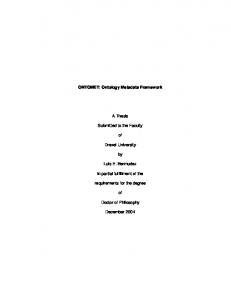
ment approaches. Figure 3 illustrates its six main steps in the most common order. Input to this process are two ontologies, which need to be aligned with one another. 1. Feature Engineering: Select small excerpts of the overall ontology definition to describe a specific entity (e.g., the label to describe the concept o1:car). 2. Search Step Selection: Choose two entities from the two ontologies to compare (e.g., o1:car and o2:automobile). 3. Similarity Computation: Indicate a similarity for a given description of two entities (e.g., simillabel (o1:car,o2:automobile)=0). 4. Similarity Aggregation: Aggregate multiple similarity assessments for one pair of entities into a single measure (e.g., simillabel (o1:car,o2:automobile) +similinstances (o1:car,o2:automobile)=0.5). 5. Interpretation: Use all aggregated numbers, some threshold and some interpretation strategy to propose the equality for the selected entity pairs (align(o1:car)=‘⊥’). 6. Iteration: As the similarity of one entity pair influences the similarity of neighboring entity pairs, the equality is propagated through the ontologies (e.g., it may lead to a new simil(o1:car,o2:automobile)=0.85, subsequently resulting in align(o1:car)=o2:automobile.
6. Iteration Input
1. Feature Engineering
2. Search Step Selection
3. Similarity Computation
4. Similarity Aggregation
5. Interpretation
Output
Figure 3: General Alignment Process Eventually, the output returned is an alignment table representing the function alignO1 ,O2 . Each of the presented steps can initialized through specific parameters. We can therefore refer to the process as a parameterizable alignment method [?], thus making FOAM a very flexible framework. In the following sections we will provide a toolbox of data structures and methods (the parameters for the process) common to many approaches that align ontologies. This gives us a least common denominator based on which concrete approaches instantiating the process depicted in Figure 3 can be compared more easily. To make the individual steps clearer the corresponding implemented activities of one specific alignment approach, namely Na¨ıve Ontology Mapping (NOM) [?], are described with each step.
6
3.1 Feature Engineering To compare two entities from two different ontologies, one considers their characteristics, i.e. their features. The features may be specific for an alignment generation algorithm, in any case the features of ontological entities (of concepts, relations, instances) need to be extracted from extensional and intensional ontology definitions. See also [?] and [?] for an overview of possible features and a classification of them. Possible characteristics include: Identifiers: Strings with dedicated formats, such as unified resource identifiers (URIs) or RDF labels. RDF/S Primitives: For example, properties or subclass relations. OWL Primitives: One entity can be, e.g., declared as being the sameAs another entity. Derived Features: These constrain or extend simple primitives (e.g. most-specificclass-of-instance). Aggregated Features: For them we need to aggregate more than one simple primitive, e.g. a sibling is every instance-of the parent-concept of an instance. Domain Specific Features: Often ontology alignment has to be performed in a specific application of one domain. For these scenarios domain-specific features provide additional value for the alignment process. Returning to our example, the relation speed is not a general ontology feature, but a feature which is defined in the automobile domain, e.g., in a domain ontology. Thus it will be important for correctly and only aligning representations of concrete vehicles. Ontology External Features: Any kind of information not directly encoded in the ontology, such as a bag-of-words from a document describing an instance, is subsumed by this class of features. We again refer to the example in Figure 2. The actual feature consists of a juxtaposition of relation name and entity name. The Car concept of ontology 1 is characterized through its label “Car”, the concept which it is linked to through subclassOf, i.e., Vehicle, its concept sibling boat, and the direct property, hasSpeed. Car is also described by its instances Porsche KA-123. The relation hasSpeed on the other hand is described through the domain Car and the range Speed. An instance would be Porsche KA-123, which is characterized through the instantiated property instance of hasOwner, Marc and the property instance hasSpeed, 250 km/h. NOM Approach: For the NOM approach we rely on identifiers and RDF/S primitives only. The complete list of used features is presented in Table 2. As already mentioned FOAM however can be easily extended with other features.
3.2 Search Step Selection Before the comparison of entities can be processed it is necessary to choose which entities to compare. The most common and obvious is to compare all entities of the 7
first ontology with all entities of the second ontology. Any pair is treated as a candidate alignment. Nevertheless it can make sense to choose or prioritize among the candidate alignments. For the integration of databases there exists a related technique called blocking [?]. A concrete approach for ontologies will be explained in one of the more advanced ontology alignment approaches later in this article.
3.3 Similarity Computation We define a similarity measure for comparison of ontology entities as a partial function as follows (cf. [?]): sim : E × E × O × O → [0, 1] Different similarity measures simk (e, f, O1 , O2 ) are indexed by the variable k. Further, we leave out O1 , O2 when they are evident from the context and write simk (e, f ). The following similarity measures are needed to compare the features of ontological entities. This list can easily be adapted and extended for additional features. For completeness we define the variable t representing the current iteration round. Object Equality: Object equality is based on existing logical assertions – especially assertions from previous iterations of our process: ( 1 alignt−1 (a) = b, simobj (a, b) := 0 otherwise Explicit Equality: This checks whether a logical assertion, such as given by the OWL sameAs primitive, already forces two entities to be equal: ( 1 iff statement(a, “sameAs00 , b), simexp (a, b) := otherwise} 0 otherwise String Similarity: Based on Levenshtein’s edit distance, ed [?], the similarity of two strings can be measured on a scale from 0 to 1 (cf. [?]). simstr (c, d) := max(0,
min(|c|, |d|) − ed(c, d) ) min(|c|, |d|)
WordNet Synonyms: Similarity measures might make use of additional external resources. This one relies on the synonym sets defined in WordNet [?]. Two strings representing synonyms return 1, otherwise 0. Set Similarity: For many features we have to determine to what extent two entity sets of entities F, G ⊂ E are similar. To remedy the problem we use the following heuristic. An entity is described by its distance to any other entity. We assume that if entities have very similar distances to all other entities, they must be very similar. We can now determine an average entity representing the set. Finally
8
we can measure the similarity of the two involved sets by applying the cosine measure: P P ~ g f ∈F f g∈G ~ simset (F, G) = P · P | f~| | g∈G ~g | f ∈F
with f~ = (sim(f, f1 ), sim(f, f2 ), . . . , sim(f, g1 ), sim(f, g2 ), . . .), ~g analogously. Dice Coefficient: Further, two sets of entities can be compared based on the overlap of the sets’ individuals[?]. Unfortunately this is only possible if the individuals are marked with a clear identifier: simdice (F, G) :=
|x ∈ (F ∩ G)| |x ∈ (F ∪ G)|
NOM Approach: The similarity computation between an entity of O1 and an entity of O2 is done by using a wide range of similarity functions. Each similarity function is based on a feature of both ontologies and a respective similarity measure as shown in Table 2 for NOM. In the first part of the table two concepts are compared. No. 1 represents that for each of the two concepts the labels are retrieved and these labels are compared using the (syntactic) string similarity.
3.4 Similarity Aggregation Our assumption is that a well thought-out combination of the so far presented features and similarity measures leads to better alignment results compared to using only one at a time. Clearly not all introduced similarity methods have to be used for each aggregation, especially as some methods have a high correlation. Even though a number of methods exist, no research paper especially focused on the combination and integration of these methods. Generally, similarity aggregation can be expressed through: P wk · adjk (simk (e, f )) simagg (e, f ) = k=1...n P k=1...n wk with wk being the weight for each individual similarity measure, and adjk being a function to transform the original similarity value (adj : [0, 1] → [0, 1]), which might yield better results. Averaging: The adjustment function adjk is set to be the identity function. Further all the individual weights are equally set to 1. As result we receive a simple average over all individual similarities: adjk (x) = id(x) wk = 1
9
Table 2: Features and Similarity Measures for Different Entity Types in NOM. The corresponding ontology is indicated through an index. Comparing Concepts
Relations
Instances
RelationInstances
No. 1 2 3 4 5 6 7 8 9 10 11 1 2 3 4 5 6 7 8 1 2 3 4 5 1 2
Feature (label,X1 ) (identifier,X1 ) (X1 ,sameAs,X2 ) relation (direct relations,Y1 ) all (inherited relations,Y1 ) all (superconcepts,Y1 ) all (subconcepts,Y1 ) (subconc.,Y1 ) / (superconc., Y2 ) (superconc.,Y1 ) / (subconc., Y2 ) (concept siblings,Y1 ) (instances,Y1 ) (label,X1 ) (identifier,X1 ) (X1 ,sameAs,X2 ) relation (domain,Xd1 ) and (range,Xr1 ) all (superrelations,Y1 ) all (subrelations,Y1 ) (relation siblings,Y1 ) (relation instances,Y1 ) (label,X1 ) (identifier,X1 ) (X1 ,sameAs,X2 ) relation all (parent-concepts,Y1 ) (relation instances,Y1 ) (domain,D1 ) and (range,R1 ) (parent relation,Y1 )
10
Similarity Measure string(X1 , X2 ) explicit(X1 , X2 ) object(X1 , X2 ) set(Y1 , Y2 ) set(Y1 , Y2 ) set(Y1 , Y2 ) set(Y1 , Y2 ) set(Y1 , Y2 ) set(Y1 , Y2 ) set(Y1 , Y2 ) set(Y1 , Y2 ) string(X1 , X2 ) explicit(X1 , X2 ) object(X1 , X2 ) object(Xd1 , Xd2 ), (Xr1 , Xr2 ) set(Y1 , Y2 ) set(Y1 , Y2 ) set(Y1 , Y2 ) set(Y1 , Y2 ) string(X1 , X2 ) explicit(X1 , X2 ) object(X1 , X2 ) set(Y1 , Y2 ) set(Y1 , Y2 ) object(D1 , D2 ), (R1 , R2 ) set(Y1 , Y2 )
Linear Summation: For this aggregation only the weights wk have to be determined. The adjk ustment function is set to be the identity function. adjk (x) = id(x) We assume that similarities can be aggregated and are increasing strictly. The weights are assigned manually or learned, e.g., using machine learning on a training set. [?] have thoroughly investigated the effects of different weights on the alignment results. In our approach we are basically looking for similarity values supporting the hypothesis that two entities are equal. If a measure doesn’t support the thesis, it still doesn’t necessarily mean that it’s opposing it. We respect the open world assumption in this paper. Further, this aggregation has the favorable characteristic that one can prove that eventually the alignments converge [?]. Linear Summarization with Negative Evidence: A negative value for wk needs to be applied if the individual similarity is not evidence of an alignment, but in contrary indicates that two entities should not be aligned. A typical example of such a case would be that super-concepts of the first entity have a high similarity with sub-concepts of the second entity. This is also included in Table 2 (No. 8 and 9 of the concepts). Sigmoid Function: A more sophisticated approach emphasizes high individual similarities and de-emphasizes low individual similarities. In the given case a promising function would be the sigmoid function, which has to be shifted to fit our input range of [0 . . . 1] (see Figure 4). 1 0,9 0,8 0,7 0,6 0,5 0,4 0,3 0,2 0,1 0 0
0,1
0,2
0,3
0,4
0,5
0,6
0,7
0,8
0,9
1
Figure 4: Sigmoid function adjk (x) = sigk (x − 0.5) with sigk (x) =
1 1+e−ak x
and ak being a parameter for the slope.
The rational behind using a sigmoid function is explained best using an example. When comparing two labels, the chance of having the same entity if only one or
11
two letters differ is very high; these might just be because of type errors or different grammatical forms. Whereas, if only three or four letters match, there is no information in this similarity at all; an aggregation of several of these low values should not lead to an alignment. High values are therefore further increased; low values are further decreased. The parameters of the sigmoid function can be regarded as an extension of the similarity methods, as they have to be adjusted according to the method simk they are applied to. Afterwards, the modified values are summed with specific weights wk attached to them. NOM Approach: NOM uses this sigmoid function for weighting its similarity measures. Further it makes use of negative evidence, as sometimes this is clearer than positive evidence.
3.5 Interpretation The approaches presented in this article are heuristics-based. An alignment is set, if the similarity indicates this. An alignment is not directly logically inferred by a reasoner as, e.g., in the work of [?]. This makes it easier to cope with limited support for or small inconsistencies in alignments – which will always be the case for real world scenarios. Therefore, from the similarity values we derive the actual alignments. We assign alignments based on a threshold t applied to the aggregated similarity measures. Further, each entity may participate in either one or multiple alignments. We use the thresholds presented in [?]. Every similarity value above the cut-off indicates an alignment; every one below the cut-off is dismissed. Constant Similarity Value: For this method a fixed constant c is taken as threshold. t=c The constant threshold seems reasonable as we are collecting evidence for alignments. If too little evidence is extracted from the ontologies, it is simply not possible to reliably present alignments from this. However, it is difficult to determine this value. One possibility is an average that maximizes the quality in several test runs. Alternatively it might make sense to let experts determine the value, which only works if the similarity value can be interpreted by them. Delta Method: For this method the threshold for the similarity is defined by taking the highest similarity value of all and subtracting a fixed value c from it. t = max(simagg (ei1 j1 , ei2 j2 )|∀ei1 j1 ∈ Oi1 , ei2 j2 ∈ Oi2 ) − c N Percent: This method is closely related to the former one. Here we take the highest similarity value and subtract a fixed percentage p from it. t = max(simagg (ei1 j1 , ei2 j2 )|∀ei1 j1 ∈ Oi1 , ei2 j2 ∈ Oi2 )(1 − p)
12
The latter two approaches are motivated through the idea that similarity is also dependent on the domain. The calculated maximum similarity can be an indicator for this and is fed back into the algorithm. At some point during the design of an alignment process one has to decide how many alignments an entity might possibly be involved: One Alignment Link: The goal of this approach is to attain a single alignment between two entities from the best similarity values. As there can be only one best match, every other match is a potential mistake, which should be dropped. Practically we do cleansing in the alignment table by removing entries with already aligned entities. A greedy strategy starts with the largest similarity values first. Ties are broken arbitrarily by argmax ˜ (g,h) , but with a deterministic strategy.
align(e, f ) ← (simagg (e, f ) > θ)∧((e, f ) = argmax(g,h)∈U ×V simagg (g, h)). Multiple Alignment Links: Often it makes sense to keep multiple alignments, e.g., if a user checks the results manually after all. In this case the interpretation can be expressed through the following formula. align(e, f ) ← sim(e, f ) > t. NOM Approach: NOM interprets similarity results by two means. First, it applies a fixed threshold to discard spurious evidence of similarity. Second, NOM enforces bijectivity of the alignments by ignoring candidate mappings that would violate this constraint and by favoring candidate alignments with highest aggregated similarity scores.
3.6 Iteration For calculating the similarity of one entity pair many of the described methods rely on the similarity input of other entity pairs. The first round uses only basic comparison methods based on labels and string similarity to compute the similarity between entities. By doing the computation in several rounds one can access the already computed pairs and use more sophisticated structural similarity measures. This is related to the similarity flooding algorithm of [?], which in contrast to our approach doesn’t interpret the edges through which the similarity is spread. Several possibilities when to stop the calculations have been described in the literature: • Fixed Number of Rounds • No More Changes to Alignments • Changes Below a Certain Threshold • Time Constraint
13
In his work [?] proved that the approach converges when certain characteristics apply to the algorithm. In specific, the weighting and aggregation function is critical in this context. Convergence can only be guaranteed if the overall similarity, i.e., the sum of all individual similarities, not just the similarities of alignments, rises monotonic and with smaller steps for each iteration. If the last change of overall similarity (increased by the sequence of estimated changes to come) is lower than the distance of any found alignment or non-alignment to the threshold, one can conclude that this gap will never be bridged, thus the alignments will not change. The iterative process can be stopped. When having more than one round of calculation the question arises if the results of each round should be converted/adjusted before they are fed back for the next round. One approach is to reuse only the similarity of the best alignments found. A possible way could be to give the best match a weight of 1, the second best of 21 , and the third of 13 . Potentially correct alignments are kept with a high probability but leave a path for second best alignments to replace them. The danger of having the system being diverted by low similarity values is minimized in this way. NOM Approach: For the first round NOM uses only a basic comparison method based on labels and string similarity to compute the similarity between entities. By doing the computation in several rounds one can access the already computed pairs and use more sophisticated structural similarity measures. Therefore, in the second round and thereafter NOM relies on all the similarity functions listed in Table 2. As we also include negative evidence in our considerations, we cannot guarantee the monotonic increase of similarity and thus convergence. But, in all our tests we have found that after ten rounds the approach converges in practice and hardly any further changes occur in the mapping table. This is independent from the actual size of the involved ontologies. NOM therefore restricts the number of runs to a fixed number.
4
Alignment Approaches
After having presented the general ontology alignment process with possible parameters we will now describe particular instantiations thereof. We start with three wellknown tools: PROMPT: PROMPT uses labels to propose alignments between two ontologies [?]. These are then merged. Anchor-PROMPT: Anchor-PROMPT adds structural evidence to this [?]. GLUE: In their approach [?] use machine learning techniques to build instance classifiers. Further they rely on the structures. Our framework FOAM comprises four approaches: Naive Ontology Mapping (NOM): NOM has already been explained along the general process in the previous section [?]. It uses a big number of different ontology features. Further, it is our baseline approach we compare all others against. Quick Ontology Mapping (QOM): This approach lies its focus on efficiency considerations of alignment algorithms [?]. 14
Active Ontology Alignment (AOA): With this approach we aim at exploiting user interaction in the best possible way. Alignment Process Feature Estimation and Learning (APFEL): For the last approach we use machine learning techniques to gain an presumably optimal alignment approach [?]. We describe all approaches along the general alignment process. Each of them has two distinct ontologies as input, and shall return the corresponding alignments.
4.1 PROMPT/Label-Approach Before presenting various advanced approaches to compute ontology alignments we present a straight forward simple approach, which is only based on the labels of the compared entities. We do this along the example of the PROMPT-tool. PROMPT [?] is a tool that provides a semi-automatic approach to ontology merging and alignment. Together with ONION [?] it was one of the first tools for ontology merging. PROMPT is available as a plug-in to the Prot´eg´e2 toolsuite. After having identified alignments by matching of labels the user is prompted to mark the alignments which should actually be merged. While merging PROMPT further presents possible inconsistencies. For this paper we concentrate on the actions performed to identify possible alignment candidates aka. the merging candidates. We do not consider the following merging steps. 1. Feature Engineering: The original PROMPT only uses labels. These could be taken e.g. from the RDFS ontology. 2. Search Step Selection: PROMPT relies on a complete comparison. Each pair of entities from ontology one and two is checked for similarity. 3. Similarity Computation: The system determines the similarities based on whether entities have similar labels. Specifically, PROMPT checks for identical labels as shown in Table 3. Table 3: PROMPT/Label: Features and Measures for Similarity Comparing Entities
No. 1
Feature (label,X1 )
Similarity Measure explicit(X1 , X2 )
4. Similarity Aggregation: As PROMPT uses only one similarity measure, aggregation is not necessary. 2 http://protege.stanford.edu/
15
5. Interpretation: PROMPT presents the pairs which have an identical label. For these pairs chances are high that they are actually the same. The user manually selects the ones he deems to be correct, which are then merged in PROMPT. PROMPT is therefore a semi-automatic tool for ontology alignment. 6. Iteration: The similarity computation does not rely on any previous computed entity alignments. One round is therefore sufficient.
4.2 Anchor-PROMPT Anchor-PROMPT [?] constitutes an advanced version of PROMPT which includes similarity measures based on ontology structures. Main changes occur for the similarity computation (step 3) and the iteration (step 6). 3. Similarity Computation: Anchor-PROMPT traverses paths between anchor points. The anchor points are entity pairs already identified as being equal, e.g., based on their identical labels. Along these paths new alignment candidates are suggested. Specifically, paths are traversed along hierarchies as well as along other relations. This corresponds to our similarity functions based on sub- and super-concepts no. 6 and 7 and other properties no. 4 in Table 2. 6. Iteration: Iteration is done in Anchor-PROMPT to allow manual refinement. After the user has acknowledged the proposition, the system recalculates the corresponding similarities and comes up with new merging suggestions. Table 4: Anchor-PROMPT: Features and Measures for Similarity Comparing Concepts
Other Entities
No. 1 4 6 7 1
Feature (label,X1 ) all (direct properties,Y1 ) all (super-concepts,Y1 ) all (sub-concepts,Y1 ) (label,X1 )
Similarity Measure explicit(X1 , X2 set(Y1 ,Y2 ) set(Y1 ,Y2 ) set(Y1 ,Y2 ) explicit(X1 , X2
4.3 GLUE GLUE [?] is an approach for schema alignment. It makes extensive use of machine learning techniques. 1. Feature Engineering: In a first step the Distribution Estimator uses a multistrategy machine learning approach based on a sample alignment set. It learns concept classifiers based on instance descriptions, i.e., their naming, or the textual content of web pages. Naturally a big amount of example instances is needed for this learning step. Further the relaxation labeling step uses features such as subsumption, frequency, etc. 16
2. Search Step Selection: date alignment.
As in the previous approaches GLUE checks every candi-
3. Similarity Computation, 4. Similarity Aggregation, 5. Interpretation: In GLUE, steps 3, 4, and 5 are very tightly interconnected, which is the reason why they are presented as one step here. From this also the alignment of concepts is derived. From the Similarity Estimator (the two learned concept classifiers) GLUE derives whether concepts in two schemas correspond to each other. Concepts and relations are further compared using relaxation labeling. The intuition of relaxation labeling is that the label of a node (in our terminology: alignment assigned to an entity) is typically influenced by the features of the node’s neighborhood in the graph. The authors explicitly mention subsumption, frequency, and “nearby” nodes. A local optimal alignment for each entity is determined using the similarity results of neighboring entity pairs from a previous round. The individual constraint similarities are summarized for the final alignment probability. The additional relaxation labeling, which takes the ontological structures into account, is again based solely on manually encoded predefined rules. Normally one would have to check all possible labeling configurations, which includes the alignments of all other entities. The developers are well aware of the problem arising in complexity, so they set up sensible partitions i.e. labeling sets with the same features are grouped and processed only once. The probabilities for the partitions are determined. One assumption is that features are independent, which the authors admit will not necessarily hold true. Through multiplication of the probabilities we finally receive the probability of a label fitting the node i.e. one entity being aligned with another one. The pair with the maximal probability is the final alignment result. 6. Iteration: To gain meaningful results only the relaxation labeling step and its interpretation have to be repeated several times. The other steps are just carried out once. The GLUE machine learning approach suits a scenario with extensive textual instance descriptions, but may not suit a scenario focused more to ontology structures. Further, relations or instances can not be directly aligned with GLUE.
4.4 Quick Ontology Mapping (QOM) When we tried to apply existing methods to some of the real-world scenarios we address in other research contributions, we found that existing alignment methods were not suitable for the ontology integration task at hand, as they all neglected efficiency. To illustrate our requirements: We have been working in realms where light-weight ontologies are applied such as the ACM Topic hierarchy with its 104 concepts or folder structures of individual computers, which corresponded to 104 to 105 concepts. Finally, we are working with Wordnet exploiting its 106 concepts (cf. [?]). When aligning between such light-weight ontologies, the trade-off that one has to face is between effectiveness and efficiency. For instance, consider the knowledge management platform built on a Semantic Web And Peer-to-peer basis in SWAP [?]. It is not sufficient
17
to provide its user with the best possible alignment, it is also necessary to answer his queries within a few seconds – even if two peers use two different ontologies and have never encountered each other before. For this purpose, we optimize the effective, but inefficient NOM approach towards our goal. The outcome is an extended version: QOM – Quick Ontology Mapping [?]. We would also like to point out that the efficiency gaining steps can be applied to other alignment approaches as well. 1. Feature Engineering: Like NOM, QOM exploits RDFS features. 2. Search Step Selection: A major ingredient of run-time complexity is the number of candidate alignment pairs which have to be compared to actually find the best alignments. Therefore, we use heuristics to lower the number of candidate alignments. Fortunately we can make use of ontological structures to classify the candidate alignments into promising and less promising pairs. In particular we use a dynamic programming approach [?]. In this approach we have two main data structures. First, we have candidate alignments which ought to be investigated. Second, an agenda orders the candidate alignments, discarding some of them entirely to gain efficiency. After the completion of the similarity analysis and their interpretation new decisions have to be taken. The system has to determine which candidate alignments to add to the agenda for the next iteration. The behavior of initiative and ordering constitutes a search strategy. We suggest the subsequent strategies to propose new candidate alignments for inspection: Random: A simple approach is to limit the number of candidate alignments by selecting either a fixed number or percentage from all possible candidate alignments. Label: This restricts candidate alignments to entity pairs whose labels are near to each other in a sorted list. Every entity is compared to its “label”-neighbors. Change Propagation: QOM further compares only entities for which adjacent entities were assigned new alignments in a previous iteration. This is motivated by the fact that every time a new alignment has been found, we can expect to also find similar entities adjacent to these found alignments. Further, to prevent very large numbers of comparisons, the number of pairs is restricted by an upper bound. This is necessary to exclude ontological artifacts such as ontologies with only one level of hierarchy from thwarting the efficiency efforts. Hierarchy: We start comparisons at a high level of the concept and property taxonomy. Only the top level entities are compared in the beginning. We then subsequently descend the taxonomy. Combination: The combined approach used in QOM follows different optimization strategies: it uses a label subagenda, a randomness subagenda, and a change propagation subagenda. In the first iteration the label subagenda is pursued. Afterwards we focus on alignment change propagation. Finally we shift to the 18
Table 5: Features and Similarity Measures for Different Entity Types Contributing to Aggregated Similarity in QOM. Features with a lower case “a” have been modified for efficiency considerations. Comparing Concepts
Relations
Instances
RelationInstances
No. 1 2 3 4 5a 6a 7a 8a 9a 10 11a 1 2 3 4 5a 6a 7 8a 1 2 3 4a 5 1 2
Feature (label,X1 ) (identifer,X1 ) (X1 ,sameAs,X2 ) relation (direct relations,Y1 ) (relations of direct superconc., Y1 ) (direct superconcepts, Y1 ) (direct subconcepts, Y1 ) (subconc.,Y1 ) / (superconc., Y2 ) (superconc.,Y1 ) / (subconc., Y2 ) (concept siblings,Y1 ) (direct instances,Y1 ) (label,X1 ) (identifier,X1 ) (X1 ,sameAs,X2 ) relation (domain,Xd1 ) and (range,Xr1 ) (direct superrelations, Y1 ) (direct subrelations, Y1 ) (relation siblings,Y1 ) (direct relation instances,Y1 ) (label,X1 ) (identifier,X1 ) (X1 ,sameAs,X2 ) relation (direct parent-concepts, Y1 ) (relation instances,Y1 ) (domain,Xd1 ) and (range,Xr1 ) (parent relation,Y1 )
Similarity Measure string(X1 , X2 ) explicit(X1 , X2 ) object(X1 , X2 ) set(Y1 , Y2 ) set(Y1 , Y2 ) set(Y1 , Y2 ) set(Y1 , Y2 ) set(Y1 , Y2 ) set(Y1 , Y2 ) set(Y1 , Y2 ) set(Y1 , Y2 ) string(X1 , X2 ) explicit(X1 , X2 ) object(X1 , X2 ) object(Xd1 , Xd2 ),(Xr1 , Xr2 ) set(Y1 , Y2 ) set(Y1 , Y2 ) set(Y1 , Y2 ) set(Y1 , Y2 ) string(X1 , X2 ) explicit(X1 , X2 ) object(X1 , X2 ) set(Y1 , Y2 ) set(Y1 , Y2 ) object(Xd1 , Xd2 ),(Xr1 , Xr2 ) set(Y1 , Y2 )
randomness subagenda, if the other strategies do not identify sufficiently many correct alignment candidates. With these multiple agenda strategies we only have to check a bounded and restricted number of alignment candidates from ontology 2 for each original entity from ontology 1.Please note that the creation of the presented agendas does require processing resources itself. 3. Similarity Computation: QOM is based on a wide range of ontology feature and heuristic combinations. In order to optimize QOM, we have restricted the range of costly features as specified in Table 5. In particular, QOM avoids the complete pairwise comparison of trees in favor of a(n incomplete) top-down strategy. The accentuated comparisons in the table were changed from features which point to complete inferred sets to features only retrieving limited size direct sets.
19
4. Similarity Aggregation: The aggregation of single methods is only performed once per candidate alignment and is therefore not critical for the overall efficiency. Therefore, QOM uses a sigmoid function with manually assigned weights in this step. 5. Interpretation: Also the interpretation step of QOM is not critical with respect to efficiency. A threshold is determined and bijectivity of alignments is maintained. The alignments have to be checked once for this. 6. Iteration: QOM iterates to find alignments based on lexical knowledge first and based on knowledge structures later. Assuming that ontologies have a fixed percentage of entities with similar lexical labels, we will easily find their correct alignments in the first iteration. We also assume that these are evenly distributed over the two ontologies, i.e., the distance in terms of links in the ontology to the furthest not directly found alignment is constant. Through the change propagation agenda we carry on to the next adjacent alignment candidates with every iteration step. The number of required iterations remains constant; it is independent from the size of the ontologies. 4.4.1
Comparing Run-time Complexity
We determine the worst-case run-time complexity of the algorithms to propose alignments as a function of the size of the two given ontologies. Thereby, we wanted to base our analysis on realistic ontologies and not on artifacts. We wanted to avoid the consideration of large ontologies with n leaf concepts but a depth of the concept hierarchy HC of n − 1. [?] have examined the structure of a large number of ontologies and found, that concept hierarchies on average have a branching factor of around 2 and that the concept hierarchies are neither extremely shallow nor extremely deep. Hence, in the following we base our results on their findings. The different algorithmic steps contributing to complexity3 are aligned to the canonical process of Section 3. For each of the algorithms, one may then determine the costs of each step. First, one determines the cost for feature engineering (feat). The second step is the search step i.e. candidate alignments selection (sele). For each of the selected candidate alignments (comp) we need to compute k different similarity functions simk and aggregate them (agg). The number of entities involved and the complexity of the respective similarity measure affect the run-time performance. Subsequently the interpretation of the similarity values with respect to alignment requires a run-time complexity of inter. Finally we have to iterate over the previous steps multiple times (iter). Then, the worst case run-time complexity is defined for all approaches by: P c = (f eat + sele + comp · ( k simk + agg) + inter) · iter 3 In
this paper we assume that the retrieval of a statement of an ontology entity from a database can be done in constant access time, independent of the ontology size, e.g. based on sufficient memory and a hash function.
20
Depending on the concrete values that show up in the individual process steps the different run-time complexities may be derived. For NOM we derive the complexity as follows. Feature Engineering is done only once in the beginning O(f eat) = O(1). Setting up the complete candidate pairs results in a complexity of O(sele) = O(n2 ), where n is the size of the ontologies. All the identified candidate pairs O(comp) = O(n2 ) will then have to be compared using features and their similarities. For this we tie the complexity of the ontology feature with the corresponding similarity measure, e.g., to compare the subconcepts of two concepts we have to retrieve and use the Set Similarity (O(setSize2 )), Ptwo subtrees (O(log(n)) 2 which makes O( k simk ) = O(log (n)). For each entity pair an aggregation operation is performed once with O(agg) = O(1). The interpretation is also done only once O(inter) = O(1). And finally with the number of iterations fixed this results in O(iter) = O(1). The worst case run-time behaviors of PROMPT, Anchor-PROMPT, GLUE, NOM, and QOM are given in the Table 6. Table 6: Complexity of Alignment Approaches O(n2 · 1) O(n2 · log 2 (n)) O(n2 ) O(n2 · log 2 (n)) O(n · log(n))
Label/PROMPT Anchor-PROMPT GLUE4 NOM QOM
4.5 Active Ontology Alignment Existing alignment approaches first identify the alignment fully automatically and then leave it up to the user to decide afterwards which ones are correct and may therefore be used in the respective application. Unfortunately it is extremely difficult to create a reasonable fully-automatic approach and even for the best approaches the results are often not satisfying. We therefore want to draw attention to a problem which hasn’t been addressed in depth yet: the proper usage of human interaction for aligning ontologies. We aim to exploit the potential of user input already during runtime of an automatic alignment process. In our approach we want to include user input in the general process during runtime. Two core questions arise: 1. At which point of the ontology alignment process is user interaction reasonable? 2. What is the user to be asked to maximally increase the quality of the alignment results? 3. How should the input affect the process parameters, i.e., should they be adjusted? 4 This
result is based on optimistic assumptions about the learner.
21
The second question is closely related to active learning approaches in machine learning [?]. The two ontologies represent the input and the correct alignments are the learning goal. Through exemplary alignments a background classifier is incrementally trained. The active learner focuses on processing those examples first which have the highest information value for building the classifier. We assume that optimization steps that can be done in beforehand have already been performed. 1. Feature Engineering: Active Ontology Alignment exploits RDF/OWL features. 2. Search Step Selection: The selection of data for the comparison process is kept simple. All entities of the first ontology are compared with all entities of the second ontology. Any pair is treated as a candidate alignment. 3. Similarity Computation: The best strategy for the similarity computation can be determined in beforehand. We will therefore simply keep the methods from the NOM approach as depicted in Table 2. 4. Similarity Aggregation: Again we use a sigmoid function with manually assigned weights in this step. 5. Interpretation: The only element dynamically changing throughout the alignment process are the automatically identified alignments themselves. We therefore want to include the user in the interpretation step during runtime. From all the calculated similarities we have received an aggregated similarity value. This value expresses the confidence that the two compared entities are the same, i.e., they can be aligned. A general threshold is set and all similarity values above the threshold automatically lead to an alignment, all below lead to a non-alignment. In this approach we further involve the user in the decision of whether an entity pair can be aligned or not. For scalability reasons it is not possible to present all the found (non-)alignments to the user for validation. However, the threshold represents a critical value, where the automatic classification has the highest doubt. Our hypothesis is that removing this uncertainty brings the biggest gains. Only alignments with this similarity value are presented to the user for validation. Further, similarities are heavily dependent on the graph structure of the ontology (see [?]): e.g., if all instances of two concepts are aligned, the concepts are most probably also to be aligned. The explicit alignment of a highly interlinked entity affects more other entities than a lowly interlinked entity. Highly interlinked entities are therefore given priority in comparison to lowly linked ones. The third question was whether to adjust the process parameters reacting to the input. This is done through changing the threshold. If the majority of answers have been positive, the threshold is set too high. For the following rounds, it is decreased according to the actual ratio of positive and negative answers. The opposite applies, if negative answers exceed their positive counterparts. The threshold is too low and
22
therefore it is increased. In practice the ratio of positives to negatives is multiplied with a fixed maximum change, which is then added or subtracted form the extant threshold. These two considerations are combined, i.e., the user is presented those automatically found alignments which are closest to the threshold value. If several alignments have the same similarity value, the highly interlinked ones are presented first. The user input for the alignment proposal is then stored with the corresponding perfect confidence of either 1 (true) or 0 (false). In the subsequent iterations they are used to calculate a new and better list of automatic alignments. 6. Iteration: The last step again doesn’t have the potential to gain from user interaction. We keep the NOM strategy.
4.6 Alignment Process Feature Estimation and Learning (APFEL) The sofar presented approaches are constricted to one of two different paradigms: Either, (i), proposals would include a manually predefined automatic method for proposing alignments, which would be used in the actual alignment process. They typically consist of a number of substrategies such as finding similar labels. Or, (ii), proposals would learn an automatic alignment method based on instance representations. Both paradigms suffer from drawbacks. The first paradigm suffers from the problem that it is impossible, even for an expert knowledge engineer, to predict what strategy of aligning entities is most successful for a given pair of ontologies. Furthermore, it is rather difficult to combine the multiple different substrategies to behave optimally. This is especially the case with increasing complexity of ontology languages or increasing amounts of domain specific conventions, which should also be included for optimal performance. The second paradigm is often hurt by the lack of instances or instance descriptions, because not in every case an ontology has many instances and in many cases instances exist only for some part of the ontology. Knowledge encoded in the intensional descriptions of concepts and relations is only marginally exploited this way. Hence, there remains the need to automatically combine multiple diverse and complementary alignment strategies of all indicators, i.e., extensional and intensional descriptions, in order to produce comprehensive, effective and efficient semi-automatic alignment methods. Such methods need to be flexible to cope with different strategies for various application scenarios. We have developed a bootstrapping approach for acquiring the parameters that drive such an approach through machine learning techniques. As a matter of fact the learned approach can be represented through a decision tree model [?]. For this approach the user doesn’t have to worry about setting the correct parameters, the system creates all this during the initial training phase. In contrast to the previous approach descriptions, we here lie our focus not on the actual parameters of the alignment approach, but on the way they are determined. In fact, we cannot even say, e.g., which concrete features are used or interpretation strategy is followed. This is assigned during a training phase. 4.6.1
Training Phase
We will now describe how the training is performed along the process in Figure 5. 23
Ontologies (O1, O2) Parameterized Alignment Method PAM (QF,QS,QW,QT)
Generation Of Initial Alignments
Initial Alignments AI
Validated Alignments AV User Validation
Generation of Feature/Similarity Hypotheses (HF, HS)
x
Feature/Similarity Combinations (DF, DS)
Training: Feature/Similarity Weighting Scheme and Threshold Fixing (DW, DT)
Representation Optimized Alignment Method (DF, DS, DW, DT)
Figure 5: Detailed Process of APFEL Generation and Validation of Initial Alignments: Machine learning as used in this paper requires training examples. Assisting the user in creating them is necessary, as in a typical ontology alignment setting there are only a small number of really plausible alignments available compared to the large number of candidates, which might be possible a priori. Presenting every candidate for validation makes the process tiring and inefficient for the human user. Therefore, we use an existing parametrization as input, e.g., QOM to create the initial alignments for the given ontologies O1 and O2 . As these results are only preliminary, we do not have to use very sophisticated processes: very basic features and similarities (e.g., label similarity) combined with a na¨ıve simple averaging and fixed threshold are sufficient in most cases. Resulting proposed pairs are stored starting with the highest probability alignments. This allows the domain user to easily validate the initial alignments and thus generate correct training data. She does not need to understand the complex ontology concepts, i.e., does not need to be an ontology engineer, but has to understand the meanings of the aligned entities. If the user further knows additional alignments she can add these alignments to the validated list. Obviously the quality of the later machine learning step depends on the quality and quantity of the validated alignments at this point. Generation of Feature/Similarity Hypotheses: The basis of the feature/similarity combinations is given by a baseline alignment method, e.g., QOM. Further, from the two given ontologies APFEL extracts additional features by examining the ontologies for overlapping features. Overlapping means that they occur in both ontologies. These might be additional features from the ontology model such as OWL primitives or special XML datatypes. At this point also domain-specific features may be integrated into the alignment process such as auto:licensenumber from an upper-level automobile ontology. These features are combined in a combinatorial way with a generic set of predefined similarity assessments including similarity measures for, e.g., equality, string similarity, or set inclusion. Table 7 illustrates this process for generating hypotheses for feature/similarity combinations. All feature/similarity combinations are added for now. Some feature/similarity combinations will not be useful, e.g., checking whether one license number is a substring of another. However, in the subsequent training step machine learning will be used to pick out those which actually improve alignment results. From the feature/similarity combinations of the arbitrary basic approach and of the extracted hypotheses we derive an extended collection of feature/similarity combi-
24
Table 7: Exemplary Features and Similarity Measures for Concepts. Comparing Concepts
No. 1 2 3 4 ...
Feature (label,X1 ) (label,X1 ) all (super-concepts,Y1 ) all (super-concepts,Y1 ) ...
Similarity Measure string equality(X1 , X2 ) string similarity(X1 , X2 ) (Y1 = Y2 ) set similarity(Y1 , Y2 ) ...
nations. Training: All validated alignment pairs are processed with the previously automatically generated collection of features and similarities. From each feature/similarity combination a numerical value is returned which is stored together with the entity pair as shown in Table 8. Further the user validation is added to the table. We can now Table 8: Training Data for Machine Learning (including user validation and value returned by each feature/similarity combination FSi ) Entity1 car auto wheel speed driver
Entity2 car automobile tire hasSpeed gear
FS1 1.0 0.7 0.0 0.7 0.2
FS2 1.0 1.0 1.0 0.0 0.0
FS3 0.8 0.7 0.8 0.0 0.0
FS4 0.0 0.0 0.0 1.0 0.0
User Grade 1 1 0 1 0
apply machine learning algorithms to the automatically generated feature-similarity pairs using the example training alignments. More specifically, the numerical values of all feature/similarity combinations are the input for the algorithm. The classification of being aligned or not represents the output. Different machine learning techniques for classification (e.g., decision tree learner, neural networks, or support vector machines) assign an optimal internal weighting and threshold scheme. Machine learning methods such as C4.5 capture relevance values for feature/similarity combinations. Feature/similarity combinations which do not have any (or only marginal) relevance values for the alignment are given a weight of zero and can thus be omitted. In a decision tree they simply are not present. With this we can set up the final ontology alignment method which we call alignoptim . Depending on the complexity of the alignment problem it might be necessary to repeat the step of test data generation (based on the improved alignment method) and training.
25
4.6.2
Runtime
2. Search Step Selection: No changes have been applied to this step. The normal procedure stays to compare all the possible alignment candidates. 1. Feature Engineering, 3. Similarity Computation: Features and the Similarity Computation have been learned during the training phase. Therefore no general description of them is possible. 4. Similarity Aggregation: No aggregation is required for the decision tree approach. 5. Interpretation: To give the reader an intuition of the results of this training step we refer to Example 4, a decision tree. Depending on the outcome of each individual feature/similarity we traverse the tree and reach a leaf indicating either that two entities are aligned (1) or not (0). FS0 0.5: 1 (32.0/1.0)
Example 4: Decision Tree Output.
6. Iteration: The iteration is again independent from the speciality of this approach. It is retained as before. In this Section 4 we have presented numerous different ontology alignment approaches. Each of them was focusing on slightly different aspects such as intuitive linguistic measures, the labels, or structural information. Further we showed ontology alignment from a perspective of efficiency or user interaction. Eventually we have presented two approaches that use machine learning techniques to come up with approaches of ontology alignment. To compare them we need to thoroughly evaluate them against each other, which is the goal of the next section.
5
Implementation and Evaluation
For the evaluation we basically take two ontologies and create alignments between the entities based on a given strategy. These alignments are validated against the correct 26
alignments which had been created beforehand. Our goal was to reach the best number of alignments, which is quantified in the f-measure (see next section). As the absolute quality of alignments is highly dependent on the complexity of the ontologies, we focus on the relative performance of different alignment strategies. The implementation itself was done in Java using the KAON2-framework5 for ontology access and maintenance. All the tests were run on a standard PC. The FOAM framework with various additional information is available through its website6 .
5.1 Set-up 5.1.1
Metrics
We use standard information retrieval metrics to assess the quality of the different approaches (cf. [?]): Recall: r =
#correct f ound alignments #all correct alignments
Precision: p =
#correct f ound alignments #all f ound alignments
F-Measure: combines the two mentioned measures. 2 f = (bb2+1)pr p+r with b = 1 being a factor to weight precision and recall. We consider the f-measure as most relevant for our evaluation since it balances well precision and recall. Further we measure the following parameters: Time: required to discover the alignments. Time consumed by the user for input is subtracted. User Validated Pairs: The number of pairs the user validates during runtime. In fullyautomatic approaches this would be 0. 5.1.2
Data Sets
Our test basis is made up of four ontology pairs, which differ in size (150 to 500 entities), modeling primitives (RDFS vs. OWL), and complexity (taxonomies vs. restrictions etc.), resulting therein that some are more suitable for full-automatic alignment than others. They have been created by hand, which is also the case for the correct alignments. These ontologies or slight adaptations thereof have already been used at the ontology alignment contests I3CON, EON, and OAEI [?, ?, ?]. The datasets are available at http://www.aifb.uni-karlsruhe.de/WBS/meh/foam/. Russia 1: In this first set we have two ontologies describing Russia. The students created the ontologies with the objectives to represent the content of two independent travel websites about Russia. These ontologies have approximately 400 entities each, including concepts, relations, and instances. The total number of possible mappings is 160, which the students have assigned manually. 5 http://kaon2.semanticweb.org/ 6 http://www.aifb.uni-karlsruhe.de/WBS/meh/foam/
27
Russia 2: The second set again covers Russia, but the two ontologies are more difficult to align. After their creation they have been altered by deleting entities and changing the labels at random. They differ substantially in both labels and structure. Each ontology has 300 entities with 215 possible mappings, which were captured during generation. Animals: The two animals ontologies are different version of one another. They contain about 40 entities each, thus being rather small examples, which might make it even more difficult to align them. The 25 alignments were provided for the I3CON contest. Bibliography: Finally, we used two ontologies from the EON contest. The basis for the contest was a bibliographic ontology provided by INRIA with 180 entities. The Karlsruhe ontology (http://www.aifb.uni-karlsruhe.de/ontology, 330 entities) is used in the Ontoweb portal. It is a refinement from other ontologies such as (KA)2. As such it does not only defines bibliographic items but many other items. About 40 alignments have been identified. One should be aware that the correct alignments are also subjective to a certain degree. Tests on manual alignments in the database community have shown an overlap of sometimes only 60% between two humans assigning them [?]. Nevertheless, for our purposes we treat them as a gold standard. 5.1.3
Strategies
We evaluated the alignment strategies described in the previous sections against each other: Labels, PROMPT: As the Label/PROMPT algorithm is rather simple and fast we use it as a baseline to evaluate the our other approaches against. NOM: Naive Ontology alignment is an approach making use of a wide range of features and measures. Therefore it reaches high levels of effectiveness and represents our quality baseline. In the first version all the similarities are then added and the average value is calculated. In the second version we used the weighting scheme based on the sigmoid function. In terms of structural information used and complexity incurred it is similar to Anchor-PROMPT. As a standard we allow 10 iterations. QOM: Quick Ontology alignment is our novel approach focusing on efficiency. We again used 10 iterations. Active Ontology Alignment For the focused semi-automatic alignment the most uncertain alignments according to our approach are presented to the user for validation. In total the user has to validate 60 entity pairs. For the smaller ontologies (Animals and Bibliography) only 20 entity pairs are provided. APFEL: We further present an approach where both the similarity aggregation and the interpretation have been left to a machine learning algorithm. We rely on eight 28
different ontology pairs and their respective correct alignments. The data has been provided for the alignment contest I3CON and EON. One of the ontology pairs was always kept back and then used for evaluation, whereas the alignments of the others were used for training. Further, we pruned the decision tree, in particular we required a minimum number of 30 objects in each leaf. Active APFEL: Finally, for completeness reasons we present an approach combing Active Ontology Alignment and APFEL. To circumvent the problem of having semi-automatic merging tools (PROMPT and Anchor-PROMPT) in our fully automatic alignment tests, we assumed that every proposition of the system is meaningful and correct. Further, as we had difficulties in running Anchor-PROMPT with the size of the given data sets, we refer to the results of the somewhat similar NOM. For GLUE we face another general problem. The algorithm has a strong focus on example instance alignments. As we can not provide this, we refrained from running the tests on a poorly trained estimator which would immediately result in poor quality results.
5.2 Results On the following pages we present the results of the different presented strategies. They are listed in Table 9. The first column mentions the used data set, the second column the used strategy. We then provide the quality measures precision, recall, and f-measure. Finally we also provide the required time.
1 f-measure 0,9 0,8 0,7 0,6 0,5 0,4 0,3 0,2 0,1 0 Labels
NOM
QOM
Active
APFEL
Figure 6: Average F-Measure Results 29
Active APFEL
Table 9: Results Data Set
Russia 1
Russia 2
Animals
Bibliography
Strategy Labels NOM QOM Active APFEL Active APFEL Labels NOM QOM Active APFEL Active APFEL Labels NOM QOM Active APFEL Active APFEL Labels NOM QOM Active APFEL Active APFEL
Precision 1.000 0.890 0.921 0.911 0.936 0.936 1.000 0.753 0.753 0.806 0.868 0.870 1.000 1.000 1.000 1.000 1.000 1.000 0.857 0.710 0.741 0.710 0.815 0.821
Recall 0.696 0.752 0.72 0.764 0.727 0.727 0.033 0.326 0.326 0.405 0.841 0.872 0.750 0.750 0.667 0.792 0.750 0.792 0.439 0.537 0.488 0.537 0.537 0.561
F-Measure 0.821 0.815 0.808 0.831 0.818 0.818 0.063 0.455 0.455 0.539 0.855 0.871 0.857 0.857 0.800 0.884 0.857 0.884 0.581 0.611 0.588 0.611 0.647 0.667
Time (ms) 47588 2869767 210052 n/a 614393 n/a 17375 485268 31636 n/a 160762 n/a 405 1853 821 n/a 1530 n/a 972 43293 2764 n/a 32026 n/a
Input 0 0 0 60 0 60 0 0 0 60 0 60 0 0 0 20 0 20 0 0 0 20 0 20
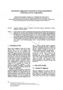
One should be aware that our core evaluation measure is the f-measure. This implies that even though some precision and/or recall may be lower for the best approach, this is only the case at the cut-off point. The average f-measure result for each strategy is depicted graphically in Figure 6. Please also note that the strategies QOM, Active Ontology Alignment, APFEL, and Active APFEL are set on-top of the NOM strategy, our default. This allows us to compare them. We now would like to draw the reader’s attention to some selected results. For all data sets labels yield the highest precision, but a considerably lower recall than all the other approaches. It seems that labels only provide nearly perfect alignments. But at the same time all the structural alignments are missed. Time is low, as we do not require more than one iteration. The structural components exploited by NOM raise recall differently according to the data sets. For some this increase is small, whereas others (see Russia 2) cannot align hardly anything without these structural components. As expected QOM is considerably faster. This is done at the cost of also lowering quality to a certain degree – always compared to our baseline NOM. Nevertheless this drop might be neglected for certain use cases. Obviously by adding user input during the alignment process, quality increases. But one still has to be aware that there might be complicated ontologies, where the user is not able to decide himself whether an align30
ment is correct or not. User input is not always capable of increasing quality, it might also decrease it. About half of the presented entity pairs were positive examples and half were negative examples, which shows that our approach finds the critical point for the highest information gain. For the optimized decision tree we again focus on the f-measure. The learned strategy is better than the standard manually trimmed NOM approach. This supports our thesis that humans cannot overview the complete complexity of ontological structures, but their knowledge in form of training data can considerably increase the performance of an alignment algorithm. Additionally, as the decision tree only requires the calculation of a subset of individual similarities, it is often faster than the other approaches. Finally our Active APFEL shows that combining the individual strategies actually leads to a better overall performance.
5.3 Lessons Learned Following the results we focus on six findings. Labels: Labels are very important for alignment, if not the most important feature of all, and alone already return very satisfying results. Semantics: The semantics of structure in ontologies can help to determine better alignments. Precision, recall, and f-measure are considerably higher for the more advanced combination methods. An average increase of 20% is achieved compared to the labels only approach. Weighting: It is especially important how to weight the individual similarities to compute an overall similarity. In the worst case results will be worse than by just using labels. Efficiency: The Quick Ontology Mapping approach shows very good results. Quality is lowered only marginally, thus supporting our hypothesis. QOM is faster than standard prominent approaches by a factor of 10 to 100 times. User Interaction: Focused semi-automatic alignment leads to better quality (+5%). Due to the large search space unfocused semi-automatic alignment doesn’t have any effect. Machine Learning: If enough training data can be provided the machine learned system is considerably better than all others, in our case the optimized decision tree. Quality increased by another 15%. And due to the structure of a decision tree it is also considerably faster than most others. Ontology alignment has different facets which can all be influenced differently. One general result of the evaluation is that there is no such thing as the absolute best ontology alignment approach. But one can see that there is much more than just comparing labels. We have provided an overview of approaches based in a very flexible parameterizable framework FOAM. In the end one has to decide which characteristics are most important: quality, efficiency, or user-interaction? And this is a task which can only be decided by the user. It is further only possible to solve when we understand what the ontology alignment is needed for in practice. 31
6
Related Work
Throughout this article we have already pointed out to related work, especially in the sections describing the process in detail (Section 3) and the alignment algorithms (Sections 4). We will just briefly mention the related approaches we have focused on. The PROMPT tool [?] was basically a tool for ontology merging based on label comparisons of the entities. Due to its plug-in functionality to Prot´eg´e, it has been very popular. It was followed by Anchor-PROMPT [?], which uses some structural features of ontologies. We also discussed GLUE[?], which originates from a more schema based view on ontology alignment. Further, the authors use machine learning techniques to improve their system. The field of ontology alignment however is not restricted to the just mentioned tools. Various authors have tried to find a general description of similarity with several of them being based on knowledge networks. [?] give a general overview of similarity, which serves as a basis for our work. Original work on alignment was presented by [?] in their tool ONION, which uses inferencing to execute mappings, but is based on manually assigned alignments or very simple heuristics, thus making it a predecessor of PROMPT. [?] created a tool for ontology alignment called Chimaera. As it is browser-based, usage is very easy. In our work we have extended and improved the approaches represented through the PROMPT-suite [?] by increasing the number of semantical features examined and GLUE by learning directly on the features rather than the underlying instances. Further, we have included additional aspects such as efficiency considerations or user interaction, which have not been addressed in any of the previous work. Whereas our work was mainly driven from practical considerations, the theoretical foundations of ontology alignment have been presented in [?]. These in turn heavily rely on work of [?] and [?]. In [?] the authors need to integrate process ontologies for industry. Interestingly they heavily rely on strict formal representations, and in their case with big success. Another work relying on formal concepts analysis is FCA-Merge [?]. An interesting approach for schema and ontology mapping is shown by [?, ?]. Explicit semantic rules are added for consideration. A SAT-solver is then used to prevent alignments to imply semantical contradictions. We however had the assumption that in most practical cases the representations will not have this exact formal representations and thus focused on similarity rather than inferencing. Logical contradictions are reflected through the negative evidence approach in our work. The Semantic Web community is nowadays broadening the focus around ontology alignment. Benchmarking considerations for ontology alignment were raised in [?]. We benchmarked our approaches following such a methodology, also considering their remarks. Further, focus is shifting from finding to executing the alignments. A proposal for a language to represent mappings was made by [?]. Ideally alignments can be presented in a language already having a corresponding inference engine as shown in [?]. Our work in this paper can be seen as a basis for these works, first we find the alignments, then we execute them. In particular we have shown in [?] that also the identification of alignments can be handed over to an inference engine. Whereas it is much more flexible in changing, e.g., the features, this approach is restricted through the capabilities of the inference engine. 32
Apart from the ontology domain research on alignment and integration has been done in various computer science fields. [?] present an approach to integrate documents from different sources into a master catalog. There has also been research on efficient schema and instance integration within the database community. [?] and [?] is a good source for an overview. In [?] existing schema alignment approaches are classified along several dimensions. It seems though, that this classification does not completely apply to our work, which often spans across several of their classes. A specific approach for schema matching was given in [?]. As ontologies are related to schemas, a lot of their work has been adapted by the ontology community. Finally, [?] give an interesting overview of up-to-date technology in the database community. However, the approaches applied in the database community normally focus on very little schema and big quantities of instances for alignment. For ontology alignment as presented in this work we need to make use of both, but we especially laid our focus on the additional semantics of the structures.
7
Concluding Remarks
Semantic alignment between ontologies is a necessary precondition to establish interoperability between agents or services using different individual ontologies. When we tried to apply these methods to some of the real-world scenarios we addressed in other research contributions [?, ?], we found that existing automatic alignment methods were not suitable for the ontology integration tasks at hand. In this article we then focused on core requirements for an ontology alignment algorithm: (i) high quality results, (ii) efficiency, (iii) optional user-interaction, (iv) flexibility with respect to use cases, and (v) easy adjusting and parameterizing. After having defined the basic terminology for this article we considered different existing and novel approaches to fulfill the mentioned requirements. Our framework for ontology alignment and mapping, FOAM, consists of a general alignment process, different instantiations of the process focusing on various aspects of ontology alignment, and the concrete implementation as a tool. We have devised the generic alignment process to investigate and compare different approaches for generating ontology alignments. In particular, we have then developed different original methods for automatically identifying alignments between two ontologies focusing on the different requirements. We have set them in contrast to other state-of-the-art algorithms with respect to quality, time consumption, and user involvement. The approaches have been presented along the simple step-by-step alignment process. Finally, the approaches have been examined in a thorough evaluation. To summarize, explicitly respecting the semantics of ontological structures increases quality considerably in contrast to na¨ıve label-based approaches. Further, it was possible to integrate efficiency or user-interaction considerations into the given framework. By using machine learning techniques we could further boost results. The approaches have thus shown an increasing level of maturity for use in a practical application scenarios. We expect that the presented findings suit semantic alignment problems for a variety of applications with many different structures.
33
Acknowledgements Research reported in this paper has been partially financed by the EU in the IST projects SWAP (IST-2001-34103), SEKT (IST-2003-506826), and the network of excellence KnowledgeWeb (EU IST-2003-507482). Many thanks to our colleagues and friends around the world for many interesting and fruitful discussions.
34