Framework for Visualizing Higher-Order Basis Functions William J. Schroeder∗
Fran¸cois Bertel†
Mathieu Malaterre‡
David Thompson§
Philippe P. P´ebay¶
Kitware
Kitware
Kitware
Sandia
Sandia
Robert
O’Barak
Saurabh
Simmetrix
Tendulkar∗∗
Simmetrix
A BSTRACT Techniques in numerical simulation such as the finite element method depend on basis functions for approximating the geometry and variation of the solution over discrete regions of a domain. Existing visualization systems can visualize these basis functions if they are linear, or for a small set of simple non-linear bases. However, newer numerical approaches often use basis functions of elevated and mixed order or complex form; hence existing visualization systems cannot directly process them. In this paper we describe an approach that supports automatic, adaptive tessellation of general basis functions using a flexible and extensible software architecture in conjunction with an on demand, edge-based recursive subdivision algorithm. The framework supports the use of functions implemented in external simulation packages, eliminating the need to reimplement the bases within the visualization system. We demonstrate our method on several examples, and have implemented the framework in the open-source visualization system VTK.
(a)
(b)
(c)
(d)
Keywords: finite element, basis function, tessellation, framework 1
I NTRODUCTION
Interpolation and approximation functions play a major role in numerical computation, simulation, and computer modeling. These basis functions take a variety of forms ranging from the linear, isoparametric shape functions found in finite element analysis to the complex non-uniform rational B-splines found in modeling and CAD applications. These functions are typically codified in small, finite subregions of a domain referred to as elements or cells. Such elements are defined by a set of maps: let R be the parametric space; each attribute, Φ : R → F may have a different type of interpolant, with geometry being a special attribute, Ξ, that has subset X ⊂ IR3 as its range and parametric coordinates (r, s,t). Typical bases range from continuous interpolants such as orthogonal Legendre, Hermite, or Lagrange polynomials seen in finite element models Φ(~r) = A0,0,0 + A1,0,0 r + A0,1,0 s + A0,0,1 t + A1,1,1 rst + · · ·
(1)
to piecewise tensor-product B-Spline basis functions defined by ni
Φ(~r) =
nj
nk
∑ ∑ ∑ Pi, j,k Nip (r)N jp (s)Nkp (t)
i=0 j=0 k=0
∗ e-mail:
[email protected] † e-mail:
[email protected] ‡ e-mail:
[email protected] § e-mail:
[email protected] ¶ e-mail:
[email protected] k e-mail:
[email protected] ∗∗ e-mail:
[email protected]
(2)
Figure 1: Results for mesh with linear geometry and cubic attribute basis functions showing (a) linear, (b) one level of uniform subdivision, (c) adaptive subdivision at 1% error, and (d) adaptive subdivision of the cubic attribute function at 0.1% error.
where p is the degree p
N (u) = ` u−u u`+p+1 −u p−1 p−1 ` u`+p −u N (u) + u`+p+1 p > 0, u ∈ [u` , u`+p+1 [ −u`+1 N`+1 (u) ` ` 1 p = 0, u ∈ [u` , u`+1 [ 0 otherwise with knot values u0 ≤ u1 ≤ · · · ≤ u p+n` +1 in IR (3) used by many CAD packages. The common thread among these is that a unique parameterization exists for the function. Furthermore, we require Ξ to be locally invertible over its domain so that f (~x) = Φ ◦ Ξ−1 (~x) exists for all ~x ∈ X. Despite the wide use of these basis functions, there is a surprising lack of tools for visualizing these functions directly, or in the case of numerical computation, the results data defined across the range of the basis function (e.g., variation of stress across an element). While methods for visualizing linear basis functions on simple computational domains (triangles, tetrahedra, quadrilaterals, and hexahedra) are quite common, methods for visualizing general higher-order basis functions are non-existent or require custom software solutions. The typical solution used today is to tessellate the basis functions with fixed levels of subdivision, and then visualize the resulting linear primitives. The reasons for this approach are compelling: first, existing visualization and graphics display systems are optimized for linear primitives, and second, implementing visualization algorithms applied to non-linear bases is an area of on-going research with few results thus far. Unfortunately, current approaches for tessellating basis functions introduces two significant problems.
First, the burden of tessellating the mesh lies outside of the visualization system. Generally the simulation package must be modified to produce output compatible with the visualization system, or a separate program is used to convert the simulation output to a form the visualization system can handle. Correctly tessellating data, in a way that is compatible across boundaries of elements and that accurately captures the results, is a difficult task. Users tend to apply uniform subdivision and over-tessellate, exacerbating the large data problem, or under-tessellate, producing significant errors in the visualization. As Figure 1 shows, poor tessellation can produce dramatically differing results. Second, as alluded to in the paragraph above, there is a decided lack of integration between simulation packages and visualization systems that becomes acutely problematic as the complexity of the basis increases. Typical visualization systems reimplement selected families of interpolation functions (e.g., linear isoparametric quadrilateral element) corresponding to supported simulation packages. While this approach works well for linear or low-order bases, for more complex functions this can be extremely difficult. For example, the modern polynomial refinement method (or p-method) for finite elements employs elaborate interpolation functions that adaptively and independently vary the interpolation order on edges, faces and regions, and may even use different interpolation bases for geometry and dependent data (i.e., the element shape versus data attributes are interpolated separately). Moreover, some numerical simulation packages use proprietary or highly optimized bases, and it is difficult if not impossible to replicate the bases in the visualization system. In this paper we address these two problems by describing a framework for automatic, adaptive basis function tessellation for bases that may be codified in external simulation packages. The framework supports any basis that is uniquely parameterized, provides the ability to add multiple tessellation error measures, and implements a simple edge-based, adaptive tessellation method. The framework has been designed so that it can be parallelized for distributed computing, and performs local, on demand tessellation of cells in response to algorithmic queries. We demonstrate the utility of the framework and show results for finite element and finite difference simulation. Finally, we have provided the implementation in the open source VTK visualization system. 2
R ELATED W ORK
In general, visualizing algorithms implemented on higher-order basis functions is an open research problem with little treatment in the literature. Much of the existing work is devoted to specific algorithms such as isocontouring or volume rendering, or is limited to basis of a particular polynomial order. Meek and Beer [15] describe a method for contour generation that tessellates the basis in parametric space, using traditional linear algorithms to produce line segments interior to the element, and then mapping the line segments back into global space. Akin and Gray [2] describe a method for generating contour lines on isoparametric finite elements by marching along a path of zero variation in isovalue, also computed in parametric coordinates (reminiscent of techniques for streamline generation). Gallagher [9] also describes methods for high precision isocontour generation in finite element meshes. Williams et al. [27] developed an accurate volume renderer that treats quadratic and linear meshes. There is no shortage of work describing basis functions for finite element application. Probably the most common formulation is the so called isoparametric element, where the interpolation function for both geometry and attribute data is of the same form [5, 12, 14, 28]. An emerging method in finite element analysis showing promise in terms of accuracy and the rate of solution convergence is known as the p-method. In this approach, the poly-
Figure 2: Overview of the framework architecture.
nomial order of interpolation across each topological entity of the element (edge, face and interior) may be independently varied as a function of desired solution accuracy [22]. While promising, the adoption of this method has been hampered due to its inherent complexity and the lack of supporting visualization tools. Basis functions are also used in modeling applications to mathematically describe the shape of objects. Coon patches, Bezier splines, non-uniform rational B-splines (NURBS), and other parametric surface descriptions are used to describe physical objects [3, 6, 7, 16]. Such basis functions have traditionally been used to represent the geometry and topology of physical objects, as in CAD/CAM application. However, these modeling basis functions can also be used to interpolate the variation in dependent variables such as stress, strain, and temperature variation. While tessellating bases for visualizing geometric models has been addressed [7], these methods are based solely on geometric considerations, including concerns on surface smoothness (i.e., continuity of derivatives). In numerical simulation both geometric and attribute data are interpolated, possibly with different bases. Thus methods that treat both simultaneously are needed. While applications of numerical simulation and modeling routinely employ higher-order basis functions, visualization systems in general support only linear bases. For example, commercial systems such as AVS [26], Data Explorer [1, 11, 13], Iris Explorer [23], and VTK [21] support a wide variety of linear types (e.g., triangle, tetrahedral, quad, hexahedra, etc.) but provide only limited support for isoparametric quadratic and infrequently, cubic, bases. 3
A PPROACH
In this section we begin by describing the framework used to implement the adaptive tessellation method. We follow this treatment with details of the tessellation procedure. In the latter part of this section we describe advanced methods to demonstrate the flexibility of the framework to support new approaches.
3.1
Adaptor Framework
A major goal of this work was to develop an architecture that would allow users to plug in their own basis functions, including providing the ability to link against external simulation packages. We wanted to avoid reproducing the implementation of the basis functions in the visualization system, or to force users to write data in a particular file format. In addition, we did not want to simply translate one data structure into another (at the cost of significantly increasing memory requirements). To realize this goal, we designed an adaptor framework residing between the existing linear visualization system (VTK in this case) and an external package. Figure 2 illustrates the key classes of the framework. The typical data visualization abstraction—that data is represented by a dataset, and in turn the dataset consists of points and cells—is preserved, except that the classes’ API removes all assumptions on the linearity of the data. The API also provides a more elaborate traversal mechanism based on cell and point iterators. These iterators are used both to traverse over the cells of the dataset, as well as on the boundaries of a cell. The representation of dependent data associated with the geometry and topology of the dataset (i.e., attribute data) is also abstracted. Access to the attribute data is via point and cell iterators; thus it is possible to associate data with any geometric or topological entity found in the dataset representation. The design defines several abstract superclasses, the GenericDataSet, GenericAdaptorCell, PointIterator, CellIterator, and GenericAttributeData that must be subclassed with concrete class implementations in order to interface to external simulation systems. The tessellation process is carried out by the GenericCellTessellator (and its subclasses). GenericCellTessellator works with the GenericSubdivisionErrorMetric and its derived classes to evaluate various types of error. Generally, these classes can be used as is, but users can create new tessellation algorithms or add new error measures to modify the default behavior of the system. A new concept that we refer to as DOF nodes was introduced into the design. These nodes represent collections of coefficients at each topological entity of a cell, excluding the cell corner vertices. For example, a triangle has four DOF nodes corresponding to its three edges and interior region. The coefficients define the interpolation function on the particular topological entity with which the DOF node is associated. Note that these coefficients may be implicitly or explicitly defined and can be omitted in many cases. The exact meaning and data structure of the coefficients depend on the particulars of the basis function being represented, and are defined by the concrete subclasses described previously. The creation of this new dataset type introduced a different API into the system, hence existing filters were no longer compatible with this new dataset. While we considered rewriting all the filters for the new API, we observed that the number of filters that operate on general datasets is relatively small, since most filters are specialized for particular types of data (e.g., images, polygon meshes). As a result, we chose the most important algorithms and rewrote them for the API introduced by the adaptor framework. These algorithms include contouring, clipping, cutting, streamline generation, glyphing, probing, extracting surface geometry, and outlining the data. A given algorithm is typically implemented as follows: for each cell c to be processed { linearDataSet = TessellateCell(c) for each linear cell cl in linearDataSet { OperateOn(cl) } }
We also created a general purpose dataset tessellator to linearize the mesh. The tessellator filter serves as a fallback position: we avoid linearizing input datasets whenever possible since doing so may consume excessive memory resources as every cell is tessellated.
With this approach, the cell tessellation is only performed when absolutely necessary, especially since we can take advantage of the iterators to visit only those cells that need processing. Further, the tessellation is performed dynamically and the results of tessellation are discarded once the processing of each cell is complete. In this way we avoid tessellating the entire dataset all it once and incurring the resulting memory cost. The remainder of this paper focuses on the tessellation algorithms used to reimplement the algorithms referred to previously. 3.2
Edge-Based Tessellation
The edge-based tessellation that we adopted is similar to [4] and [19]. Besides the design of our framework, our major contributions have been to use a more sophisticated error metric, to add additional efficiencies into the algorithm, and to introduce advanced methods for tessellation. We describe the basic algorithm in this section, and discuss the error metric in the next. Finally, we describe some advanced tessellation methods to demonstrate the flexibility of the adaptor framework. The central idea behind the algorithm is simple: each cell edge is evaluated via an error metric and may be marked for subdivision. Based on the cell topology, and the particular edges requiring subdivision, templates are used to subdivide the cell. This process continues recursively until the error metric is satisfied on all edges. This algorithm is easily implemented in 2D, but in 3D maintaining face compatibility is an issue and is discussed later in this section. There are also several performance issues to consider as well, including minimizing the cost of evaluating the error metric. The advantages of this algorithm are its relative simplicity, and the fact that cells can be tessellated independently. This is because edge subdivision is a function of one or more error measures that consider only information along the edge, and do not take into account cell information. Therefore no communication across cell boundaries is required, and the algorithm is well suited for parallel processing and on the fly tessellation as cells are visited during traversal. 3.2.1
Details
The algorithm operates on topological simplices sni of dimension n that form a compatible mesh M: M=
[ i
sni
(4)
The mesh is compatible meaning that simplices intersect only on p boundary faces fk of dimension p p
p
p
n m n sm i ∩ s j = f k with p < min(m, n) and f k ⊂ si , f k ⊂ s j
(5)
Here we refer to the sni as cells, and note that cells of non-simplicial topology can be treated by first triangulating them, insuring that the resulting tessellation is compatible. Also, the algorithm supports meshes whose cells are of mixed dimension n. The algorithm operates on M to produce a linear (both in geome¯ In the discussion that try and topology), compatible tessellation M. p follows we distinguish between mesh topological entities fk (i.e., vertices, edges, faces, regions) and tessellant topological entities p p f¯k . Obviously f¯k are produced from the tessellation of sni . Edges are subdivided once when the error metric fails. As described later in this section, the error metric E consists of multiple error measures εi , and if any one exceeds its error threshold εiT the edge is split Split edge e if εi > εiT , for any εi ∈ E
(6)
2
2
C
2
attribute 5
4
0
5
4
1 0
5
α
4
1 0 3
3
(a) case 001
(b) case 011
(c) case 111
Currently the subdivision splits the edge at the parametric midpoint. In the future we may optimize the split position to minimize the error. After all edges are evaluated, the cell is assigned a case number. The case number indexes into a subdivision table as illustrated in Figure 3. The triangle is then subdivided and the process continues.
Face Consistency in 3D
The algorithm requires special treatment when tessellating the faces of 3D cells. Referring to Figure 3(b), notice that there are two different ways to tessellate the triangle (the face of a tetrahedron) as indicated by the dotted line. While the method of ordered triangulation [20] can be used to address this situation, we wanted a faster method specialized to tetrahedra. Ignoring any geometric criteria used to select the diagonal, we instead use strictly topological deciders. In this case point ids were used, under the assumption that the cell point ids are unique and can be sorted. The rule here is that the diagonal edge connecting the lowest point id is selected. (This is similar to the work of [17].) In practice we use two subdivision case tables depending on whether the tetrahedron is a left-handed or right-handed. A righthanded tetrahedron is one in which the ordering of its indices {0, 1, 2, 3} is such that the first three indices define a face with an inward pointing normal (using the right-hand rule). A left-handed tetrahedron produces an outward pointing normal. Each table consists of 26 = 64 entries where each entry defines the tetrahedra to be created during subdivision. We decided to use two tables for efficiency rather than a single table with symmetric modifiers as in [19]. 3.2.3
Efficiency Considerations
Evaluation of the edge error metric can be a time consuming operation. Further, since many cells may share the same edge, a naive implementation of the algorithm repeatedly evaluates the error metric many times. Additional costs are associated with edge splitting including coordinate system conversion and evaluation of the attribute data at the center split point. To improve the performance of the algorithm, we devised a special hash table to store information on edges to insure that calculations are performed only once. The hash table also stores point ids which are essential for insuring proper face consistency in 3D as described previously. The hash table is specially designed to retain edge information only as long as it is needed. For example, consider a mesh consisting of two higher-order triangles joined along a common mesh edge e. Then all tessellant edge information produced along e must be maintained after the first triangle is processed because successful processing of the second triangle also requires information along e. It is only after the second triangle is processed that the information associated with e can be deleted. In 3D, tessellant edge information on the faces of cells must also be maintained until the adjoining face neighbor (if any) is processed.
am a1 ai
1
3
Figure 3: A portion of the subdivision case table.
3.2.2
d
B
D
A
a
0
t 0
(a)
0.5
1
(b)
Figure 4: Definition of the geometric and attribute error measures.
Memory management via reference counting was used to implement this capability. Edges, when constructed during tessellation, must be classified in the interior, on the edges, or on the faces of the original higher-order cell. Tessellant edges have an initial reference count equal to the number of times the higher-order topological entities on which they are classified are used in the mesh. Once a cell is processed, it decrements the reference count of all the edges created during tessellation. Thus all interior edges are immediately deleted, and tessellant edges on the boundary of the cell may or may not be deleted depending on whether all neighboring cells have been processed. Assigning an initial reference count depends on proper classification of edges. One way to achieve this is to create a richer topological structure where tessellant vertices, edges and faces keep track of their relationship to each other, as well as their relationship to the original cell. We decided against this approach due to the costs associated with memory management. Instead, we deduce the classification of edges from either geometric or topological information. Edges can be classified using geometric calculations, with minimal impact on memory requirements, by determining (in parametric space) whether the edge is located along a cell edge, on a cell face, or interior to the cell. This works well as long as numerical accuracy concerns can be avoided (e.g., by limiting the depth of recursive tessellation). Alternatively, topological information can be used to classify edges. In this case, a classification is carried by each tessellant vertex. The classification is simply a label that indicates the type and on which topological entity the vertex lies (e.g. which mesh vertex, edge, face, or region). Then the classification of any tessellant edge is a simple table lookup based on the topology of the cell and the classification of the edges vertices. Of course, any vertices created during subdivision receive the classification of the tessellant edge as it is subdivided. 3.3
Error Measures
What makes this algorithm adaptive is that edge splitting is controlled by local mesh properties and/or its relation to the view position. The goal is to insure that the quality of the tessellation is consistent with the particular requirements of the visualization. In general, we expect the adapted tessellation to be of better quality as compared to a fixed subdivision for the same number of simplices, or have fewer simplices for tessellations of equal quality. Our design allows for the definition of multiple error measures. As indicated in Equation 6, the error metric consists of several error measures, each of which evaluates local properties of the edge against the linear approximation, and compares the measure against a user-specified threshold. If any measure exceeds the threshold, then the edge is subdivided. These error measures may evaluate geometric properties, approximation to solution attributes, or error related to the current view, among other possibilities. Error measures based on geometry or attributes are independent of view and the mesh requires only one initial tessellation. The following paragraphs describes several error measures that
we have found useful. Since the tessellator is designed to process a list of error measures, it is straightforward to add new ones (by deriving from the GenericSubdivisionErrorMetric class) and/or combine it with existing error measures.
A 4
2 2
0
−2
y
Attribute-Based Error Measure. Referring to Figure 4(b), this error measure is the distance between the linearly interpolated value ai of an attribute at the midpoint and the actual value of this attribute at the edge midpoint am . Image-Based Geometric Error Measure. This error measure is the distance, in pixels, between the line (AB) projected in image space to the midpoint C also projected in image space. Because the computation involves projection through the current camera matrix, this error measure is view-dependent. As a result, the tessellation may be crude in portions of the mesh away from the camera. Note that one of the disadvantages of this approach is that tessellation may be required each time the camera is repositioned relative to the mesh. 3.4
Advanced Methods
In the first half of this section we described a basic algorithm focused on speed and simplicity. In this section we describe an alternate tessellation method to demonstrate the utility of the framework. (Details on these methods are available in [24] and additional research is ongoing.) This advanced method focuses on two requirements: guaranteeing that the tessellation captures all topological features of the higher order bases, and producing a refined mesh with high-quality elements. We address these topics in the following subsections. 3.4.1
Capturing Topological Features
To capture all the features of the original higher-order basis, certain conditions must be met on the tessellation. Often these conditions depend on the characteristics of a visualization algorithm. For example, linear isocontouring algorithms require that the following conditions are met in order to produce topologically correct results. • each mesh edge intersects an isocontour of a particular value at most once, • no isocontour intersects a mesh face without intersecting at least two edges of the face, and • no isocontour is completely contained within a single element. By definition, these conditions are directly related to critical points, since an extremum of a differentiable1 Φ over an open domain is necessarily a critical point. Linear meshes assume that all extrema of the scalar field Φ : IR3 → IR occur at vertices, but in general when using a higher-order basis this is not the case, and extrema can be found interior to a cell. These three requirements above may be rephrased in terms of critical points: 1 we
assume the field is differentiable over each cell.
−4
−6
−2
0
C D
6
B
x
−6
4
Object-Based Geometric Error Measure. Referring to Figure 4(a), this error measure is the perpendicular distance, d, from the edge center point C to the straight line passing through the cell edge vertices (A and B). Note that d is computed in world coordinates, but C is computed by evaluation at the parametric center of the edge. The perpendicular distance is used rather than the distance between C and D because if C lies on (AB) but is not on D the error is non-zero and may produce many useless edge subdivisions. Object-Based Flatness Error Measure. This error measure is the angle between the chords (AC) and (CB) passing through the real mid-point C. As the angle approaches 180° the edge becomes flat. The threshold is the angle over which the edge is viewed as flat.
−4
4
2
C B
0 −2
D
−4
A −6
−4
−2
y
0
−6 2
4
6
−8
x Figure 5: Critical points must be connected into a proper tessellation.
(C1) Φ has no interior extrema along any tessellant edge f¯k1 . We may specify an edge as a linear relationship among parametric coordinates so that, if the dependency is in terms of r, this constraint may be written g0 (r) = ( ∂∂Φr + a ∂∂Φs + b ∂∂tΦ )(r,s(r),t(r)) 6= 0 over some interval ]r0 , r1 [⊂ IR, where a and b are real constants. Note that one can have g0 (r) = 0 (i.e., an extrema on f¯k1 ) even though ∇Φ(r,s(r),t(r)) 6= 0. (C2) Φ has no interior extrema over any tessellant face f¯k2 . We may specify a face as a linear relationship among parametric coordinates so that this constraint may be written, if the dependency is that of t in terms of r and s, ( ∂∂Φr + a ∂∂tΦ , ∂∂Φr + b ∂∂tΦ )(r,s,t(r,s)) 6= 0 over some open domain Ui ⊂ IR2 , where a and b are real constants. Once again, this expression can vanish (i.e., both components are 0) even at a point where ∇Φ does not. (C3) Finally, we note that for a component of an isocontour to be completely contained in some element, a critical point of the differentiable Φ must exist somewhere in the element. Thus, we must insure that all extrema must occur at vertices. In order to meet these requirements, it is clear that we must locate all critical points on the interior of the element, as well as critical points of Φ restricted along each f¯ki . Once located, these critical points must be inserted into an initial tessellation of the element in a way that preserves the properties described above2 . For example, consider a d-dimensional finite element with a set of d + 1 or more ∗ } ∈ Rm+1 . There is no guarantee that an critical points {r0∗ , r1∗ , . . . , rm i edge ru∗ rv∗ should exist in the tessellation. As Figure 5 illustrates in two dimensions, the restriction of Φ to the interior of ru∗ rv∗ may have some critical point that is not a critical point of Φ. For instance, if edge AC were used instead of edge BD, there is some isovalue Φ(X) < Φ(A) along edge AC that would not appear in the output since Φ(X) < Φ(A) < Φ(C). Thus isosurfaces generated by ABC and ACD would not be topologically correct, while those generated by ABD and BCD would be correct. In fact, this means that the tessellation of the initial cell vertices along with volume, face and edge critical points must comply with (C1). In general, for an edge 2 Because this initial tessellation then serves as an input to the edgesubdivision algorithm, edge refinement will not miss features interior to an element
to be present in the initial tessellation of an element, there should be a path of steepest descent (or ascent) that connects its endpoints. Faces and non-isolated critical introduce additional complexity. Some tessellant faces(i.e., triangles) ru∗ rv∗ rw∗ should not be in the final tessellation because they may cross curves that induce a minimum or maximum on the restriction of Φ to the face—this means that the choice of subfaces is constrained by (C2). This is further complicated when non-isolated critical points are allowed. Isosurfacing algorithms allow edges or faces to be composed of critical points, while curves and sheets of critical points are not allowed interior to an element. An initial tessellation that meets the above requirements will guarantee that linear isosurfacing algorithms will produce topologically valid approximations3 . Even without properly connecting the critical points, the true range of Φ over R will be represented, which is perhaps the most basic characterization of Φ possible. However, it is possible that other visualization algorithms make assumptions beyond the ones considered above. For example, some volume rendering algorithms assume that scalar values along a ray passing through an element are constant or linear (even though trilinear interpolants do not meet this criterion except along a coordinate axis). Specific visualization algorithm requirements must be considered when developing an initial tessellation. The framework supports this by allowing each class representing a type of cell to present an initial tessellation to the tessellation algorithm. This initial tessellation may be altered depending on the requirements at hand. 3.4.2
R ESULTS
In this section we use our framework to visualize several datasets to demonstrate its effectiveness. The framework code is integrated into VTK and available for download from vtk.org. Note that in Sections 4.1 through 4.3, adaptors to Simmetrix, Inc.’s (simmetrix.com) proprietary commercial system were used to process the datasets shown. In Section 4.4, adaptors to Sandia’s S3D simulation system were used. 4.1
(b)
(c) Figure 6: Results showing (a) linear, (b) one level of uniform subdivision, and (c) adaptive subdivision.
or performing one level of fixed subdivision ((Figure 1(b)) compares to adaptive methods (Figures 1(c) and (d)). Note that Figures 1(a) and (b) are typical of what current visualization systems produce.
Refined Element Quality
Although visualization algorithms are generally less susceptible to simplices of poor quality than finite element simulations, there are many instances in which poor element quality can be problematic. For example, hardware interpolation across a long, thin triangle can introduce artifacts during rendering. To ensure a high-quality tessellation, there are various approaches that can be used to improve quality. One simple, effective approach in 3D is to simply select the best, alternative tessellation of a tetrahedra that does not affect the triangulation on its faces. This choice is due to the fact that certain configurations of edge subdivision may be tessellated in more than one way. The framework supports quality-driven tessellation by separating the adaptive tessellation functionality into a class of its own. Implementing this capability (or other tessellation scheme) requires deriving from the GenericCellTessellator class (see Figure 2). 4
(a)
Mesh Linear One Subdivision Adaptive (1.0% error) Adaptive (0.1% error)
3 We
can further extend linear isosurfacing algorithms to find zeros of the higher-order interpolant rather than the linear one so that the piecewise approximation of the isosurface will be exact at each output vertex.
Points 86 524 4,901 177,348
Cells 293 2,344 22,892 925,761
Table 1: Results for Figure 1.
4.2
Quadratic Geometry, Quadratic Attribute
The next example is a finite element mesh with quadratic geometric and attribute basis functions. The attribute data is an approximation to the analytic function f (x, y, z) = y2 + z2 + 10(1 − x). Figure 6 compares how visualizing the mesh as linear elements (Figure 1(a)) or performing one level of fixed subdivision ((Figure 1(b)) compares to the adaptive method. For the adaptive method, a flatness error measure of 177° and error of 0.1% in the attribute value was used. Mesh Linear One Subdivision Adaptive
Time (secs) 0.08 0.22 9.56
Points 415 2,440 98,797
Cells 1,227 9,816 482,487
Table 2: Results for Figure 6.
Linear Geometry, Cubic Attribute
The first example is a finite element mesh with linear elements and cubic attribute functions (the Kovasznay flow problem). Figure 1 compares how visualizing the mesh as linear elements (Figure 1(a))
Time (secs) 0.03 0.06 0.44 18.2
4.3
Error Measures
The third example compares the effect of different error measures on the adaptive tessellation process. As Figure 7 shows, a plate with a hole is represented by a finite element mesh. Both the geometry and attribute data are interpolated with quadratic basis func-
tions. The attribute field is an approximation to the analytic function f (x, y, z) = 100(100x2 + 100y2 + z). For comparison purposes, the mesh is uniformly subdivided (three levels of subdivision) and the resulting error in geometry and attribute data is used to specify the error thresholds for the adaptive process. The geometric error metric threshold is set to 2.7% of the diagonal of the bounding box of the mesh. The attribute error metric threshold is set to 2.04% of the attribute range. The flatness error metric threshold is set to 160.5°. Table 3 compares the number of points and cells created in each case. One of the more gratifying aspects of these results is that for equivalent error measures, the adaptive subdivision produces fewer linear primitives in faster time than the uniform subdivision. When combining all the error measures (item #7 in Table 3), the adaptive process ran nearly 20 times faster, and produces 34 and 50 times fewer points and cells, respectively, than the fixed subdivision of equivalent quality. Mesh Original (1) Fixed (2) Flatness (3) Geometric (4) Attribute (5) Flat. + attr. (6) Geom. + attr. (7)
Time 0.01 0.87 0.0166 0.022 0.034 0.04 0.045
Points 82 19,612 164 264 377 480 569
Cells 200 102,400 373 695 1,418 1,722 2,035
(a)
(b)
(c)
(d)
(e)
(f)
(g)
(h)
(i)
(j)
Table 3: Adaptive versus fixed subdivision for varying error measures. (1) Original higher order mesh, (2) fixed subdivision,(3) flatness error metric only, (4) geometric error metric only, (5) attribute error metric only, (6) flatness and attribute error metrics, and (7) combined geometric and attribute error metrics.
4.4
Quadratic Isocontouring
One application of higher order visualization is the identification of features in complex flow simulations. In particular, Figure 8 shows isocontours of the vorticity magnitude of a channel flow computed with a 3-dimensional finite difference scheme using Sandia’s S3D simulation package for turbulent reacting flows. To produce the isocontours, we adapted a 3 × 3 × 3 quadratic finite difference stencil to the framework (Figure 9(b)). This contrasts with the traditional approach of using trilinear interpolants for visualizing the results of such finite difference simulations (Figure 9(a)). It is not clear what the best interpolant is to represent such high order (up to order 12 in each direction) finite difference solutions. However, by inspecting differences in visualization results when employing interpolants of different orders, we gain additional information about how the simulation is behaving. 5
C ONCLUSION AND F UTURE W ORK
We have developed a general, flexible framework supporting the automatic tessellation of higher-order basis functions. The framework supports cells that may employ different basis functions for the interpolation of geometry and attribute data. By using an abstract, adaptor-based architecture the framework may be extended by adding new classes or derivation, and can be linked against external simulation packages avoiding the need to duplicate data structures or convert data files. An error metric has been defined that consists of a set of measures for geometry, data attribute and view error, which may also be extended by object derivation. The error metric controls an efficient, edge-based, recursive subdivision algorithm that can produce compatible tessellations on demand during
Figure 7: Adaptive versus fixed subdivision: (a,b) fixed subdivision, (c,d) combined geometric and attribute error metrics, (e,f) geometric error metric only, (g,h) flatness error metric only, and (i,j) attribute error metric only.
R EFERENCES
Figure 8: Isocontour of the vorticity magnitude of a channel flow computed with a 3-dimensional finite difference scheme.
(a)
(b)
Figure 9: Differences between linear (a) and quadratic (b) isocontours of the same underlying finite difference simulation. Note the differences in topology. (Dataset courtesy of A. Gruber (SINTEF).)
algorithm execution. The framework supports advanced techniques such as pre-tessellation for critical points and the ability to control mesh quality by selecting the best tessellations during the subdivision process. We are currently working on improving the speed of the tessellation process and investigating alternative error measures. In particular we continue to work on improving the quality of the adapted mesh. This is especially challenging since the input to the algorithm often consists of poorly shaped cells, and we want to insure that any cells that we generate are of equal or better quality than the input. ACKNOWLEDGEMENT This work was supported by the NSF under SBIR Phase II grants DMI-0128453 (Kitware) and DMI-0132742 (Simmetrix), and by Sandia National Labs under grant B527065. Authors affiliated with Sandia were supported by the United States Department of Energy, Office of Defense Programs. Sandia is a multiprogram laboratory operated by Sandia Corporation, a Lockheed-Martin Company, for the United States Department of Energy under contract DE-AC0494-AL85000.
[1] G. Abram and L. Treinish. An extended data flow architecture for data analysis and visualization. In Proc. of Visualization ’95, pages 263–269. IEEE Computer Society Press, October 1995. [2] J. E. Akin and W. H. Gray. Contouring on isoparametric elements. Int. J. of Numerical Methods in Engineering, 11:1893–1897, 1977. [3] P. Burger and D. Gillies. Interactive Computer Graphics Functional, Procedural, and Device-Level Methods. Addison-Wesley, 1989. [4] A. J. Chung and A. J. Field. A simple recursive tessellator for adaptive surface triangulation. J. Graphics Tools: JGT, 5(3):1–9, 2000. [5] R. D. Cook, D. S. Malkus, and M. E. Plesha. Concepts and Applications of Finite Element Analysis. John-Wiley, third edition, 1989. [6] G. Farin. Curves and Surfaces for Computer Aided Geometric Design. Academic Press, 1990. [7] I. D. Faux and M. J. Pratt. Computational Geometry for Design and Manufacture. Ellis Horwood, 1979. [8] P. J. Frey and P.-L. George. Mesh Generation. Hermes Science Publishing, Oxford & Paris, 2000. [9] R. S. Gallagher and J. C. Nagtegaal. An efficient 3-d visualization technique for finite element models and other coarse volumes. Computer Graphics, 23(3), July 1989. [10] B. Haasdonk, M. Ohlberger, M. Rumpf, A. Schmidt, and K. G. Siebert. Multiresolution visualization of higher order adaptive finite element simulations. Computing, 70(3):181–204, July 2003. [11] R.B. Haber, B. Lucas, and N. Collins. A data model for scientific visualization with provisions for regular and irregular grids. In Proc. of Visualization ’91, pages 298–305. IEEE Comp. Soc. Press, 1991. [12] J. R. Hughes. The Finite Element Method: Linear Static and Dynamic Finite Element Analysis. Prentice-Hall, 1987. [13] IBM Corp. Data Explorer Reference Manual, 1991. [14] L. Lapidus and G. F. Pinder. Concepts and Applications of Finite Element Analysis. John-Wiley, 1982. [15] J. L. Meek and G. Beer. Contour plotting of data using isoparametric element representations. International Journal of Numerical Methods in Engineering, 10:954–957, 1974. [16] M. .E. Mortenson. Geometric Modeling. John Wiley & Sons, 1985. [17] G. Nielson and J. Sung. Interval volume tetrahedrization. In Proc. of Visualization ’97, pages 221–228. IEEE Comp. Soc. Press, 1997. [18] P. P. P´ebay and D. Thompson. Communication-free streaming mesh refinement. Journal of Computing and Information Sciences In Engineering, 2005. In print. [19] D. Ruprecht and H. M¨uller. A scheme for edge-based adaptive tetrahedron subdivision. In H.-C. Hege and K. Polthier, editors, Mathematical Visualization, pages 61–70. Springer Verlag, Heidelberg, 1998. [20] W. J. Schroeder, B. Geveci, and M. Malaterre. Compatible triangulations of spatial decompositions. In Proc. of Visualization 2004, pages 211–218. IEEE Computer Society, 2004. [21] W. J. Schroeder, K. M. Martin, and W. E. Lorensen. The Visualization Toolkit An Object-Oriented Approach To 3D Graphics. Prentice-Hall, third edition, 2004. [22] M.S. Shephard, S. Dey, and J. E. Flaherty. A straightforward structure to construct shape functions for variable p-order meshes. Computer Methods in Applied Mechanics and Engineering, 147:209–233, 1997. [23] Silicon Graphics, Inc. Iris Explorer User’s Guide, 1991. [24] D. Thompson, R. Crawford, R. Khardekar, and P. P´ebay. Visualization of higher-order finite elements. Technical Report SAND2004-1617, Sandia National Laboratories, 2004. [25] D. C. Thompson and P. P. P´ebay. Performance of a streaming mesh refinement algorithm. Sandia Report SAND2004-3858, Sandia National Laboratories, August 2004. [26] C. Upson, T. Faulhaber Jr., D. Kamins, et al. The application visualization system: A computational environment for scientific visualization. IEEE CGA, 9(4):30–42, July 1989. [27] P. L. Williams, N. L. Max, and C. M. Stein. A high accuracy volume renderer for unstructured data. IEEE Transactions On Visualization and Computer Graphics, 4(1), January 1998. [28] O.C. Zienkiewicz and R.L. Taylor. The Finite Element Method – Volume 1. McGraw-Hill Book Co., 4th edition, 1987.