ization plays an important role in object detection, which also contains a ... can discriminate a dog against other objects or backgrounds. Bag of the visual words ...
Free-Shape Subwindow Search for Object Localization Zhiqi Zhang, Yu Cao, Dhaval Salvi, Kenton Oliver, Jarrell Waggoner, and Song Wang Department of Computer Science and Engineering, University of South Carolina, Columbia, SC 29208, USA {zhangz, cao, salvi, oliverwk, waggonej, songwang}@cec.sc.edu Abstract Object localization in an image is usually handled by searching for an optimal subwindow that tightly covers the object of interest. However, the subwindows considered in previous work are limited to rectangles or other specified, simple shapes. With such specified shapes, no subwindow can cover the object of interest tightly. As a result, the desired subwindow around the object of interest may not be optimal in terms of the localization objective function, and cannot be detected by a subwindow search algorithm. In this paper, we propose a new graph-theoretic approach for object localization by searching for an optimal subwindow without pre-specifying its shape. Instead, we require the resulting subwindow to be well aligned with edge pixels that are detected from the image. This requirement is quantified and integrated into the localization objective function based on the widely-used bag of visual words technique. We show that the ratio-contour graph algorithm can be adapted to find the optimal free-shape subwindow in terms of the new localization objective function. In the experiment, we test the proposed approach on the PASCAL VOC 2006 and VOC 2007 databases for localizing several categories of animals. We find that its performance is better than the previous efficient subwindow search algorithm.
1. Introduction An important task in computer vision and image understanding, object localization tries to solve the following problem: given that there are a known number of specific objects in an image, find the exact locations of the objects in the image. In most cases, we are only interested in localizing one object of interest from an image. Object localization plays an important role in object detection, which also contains a recognition step to determine whether the object of interest is present in an image and how many instances of the object are in an image. Many object detection systems carry out object localization first by hypothesizing that the object of interest is present in an image, followed
by a recognition step [14, 9, 27, 19], which verifies whether the located object is the desired object of interest. In many applications [10, 11, 15, 6, 24, 7], the recognition step must additionally compare the localization results from hypothesizing different objects in the image. This paper is focused only on the object localization problem. In computer vision, object localization is often a very challenging problem because an object to be localized actually defines a category of objects with large intra-category variations. For example, given an image that contains a dog, we want to localize this dog accurately. While we know there is a dog in this image, we do not know its species, size, pose, and color. This usually requires a supervised learning process to extract some common features from all dogs that can discriminate a dog against other objects or backgrounds. Bag of the visual words is the state-of-the-art technique developed for achieving this goal. It can detect a set of features points from an image and associate each feature to a specific score that reflects its likeliness of being a feature of the desired object. For example, a positive-score feature is likely to be on the object of interest while a negative-score feature is unlikely to be on the object of interest. In this case, object localization can be reduced to searching for a subwindow that covers as many positive-score features and as few negative-score features as possible. Sliding window [2, 7, 8, 5] is a widely used technique for addressing this problem: for every possible subwindow in an image, check the feature scores covered by the window, and select the one with the maximum total feature scores as the optimal subwindow to localize the object of interest. Without knowing the size and the pose of the object, this technique must check subwindows with different sizes, which is computationally expensive. To reduce the size of the search space, only rectangular subwindows, with four sides parallel to the four sides of the image, are searched in the sliding window technique. Recently, more efficient branch and bound algorithms [13, 1] have been developed to speed up the subwindow search without exhaustively checking all possible subwindows while keeping the global optimality of the result. In these efficient subwindow search
(ESS) algorithms, the searched subwindows are also rectangles as in the sliding window technique. As illustrated in Fig.1(a), a rectangular subwindow may not cover the object of interest tightly. As a result, the desirable subwindow, shown in green in Fig.1(a), may cover many negative-score features and therefore may not be detected as the optimal subwindow, which is shown in pink in Fig.1(a).
(a)
timal free-shape subwindow in terms of the new localization objective function. Note that, although we consider edge information in our formulation, we are not attempting to address the challenging problem of object segmentation as in [23] and [18]. While a successful segmentation automatically leads to a perfect localization, even the state-of-the-art segmentation methods only work on images where an object class shows relatively small variations (in texture, color, pose, species, occlusion, etc.) within relatively simple and consistent backgrounds. As in ESS, this paper is aimed at localizing objects from a large number of images, such as the entire VOC dataset, with very complex object variations and different backgrounds.
(b)
Figure 1. An illustration of the problems of object localization by searching for (a) rectangular subwindows, and (b) polygonal subwindows without other constraints. Red and blue dots in the images indicate the positive-score and negative-score features, respectively.
Recently, Yeh et al. [26] extended the ESS algorithms to search for polygonal subwindows that may not be rectangular. However, the shape of the subwindow must be pre-specified, such as a polygon with a specified number of sides or a polygon formed by stacking multiple rectangles. A non-rectangular subwindow has more degrees of freedom than a rectangular subwindow. This would substantially increase the computational complexity of the optimal subwindow search. More importantly, by allowing a more complex shape for the searched subwindow, the resulting object localization algorithm may be very sensitive to the noise of the detected features and derived feature scores. An example is shown in Fig.1(b), where we search for a pentagon subwindow. We can see that even a single positive-score outlier feature in the background may lead to a undesirable optimal subwindow (shown in pink) with a highly irregular shape. In this paper, we develop a new graph-theoretic approach for object localization where the searched subwindow can take any shape, e.g. a free-shape polygon without a specified number of sides. To address the problem of being sensitive to the feature noise, we additionally require the resulting subwindow to align well with edge pixels detected from the image. This way, the new localization objective is formulated as searching for a free-shape subwindow by striking a balance between two goals: (a) the optimal subwindow should cover as many positive-score features and as few negative-score features as possible, as in the previous methods, and (b) the sides of the optimal subwindow should have the maximum coincidence with the detected image edge pixels. In particular, we define a localization objective function in a ratio form and show that the ratiocontour graph algorithm [22] can be adapted to find the op-
2. Bag of Visual Words and Rectangular Subwindow Search for Object Localization Object localization that combines the rectangular subwindow search and the bag of visual words technique usually consists of following steps [13]. First, a set of training images that contain the object of interest are collected, and the ground-truth object localization is manually constructed for these training images. Here the ground-truth object localization is the tightest rectangular subwindow (with four sides parallel to the four sides of the image) that fully covers the object of interest, as illustrated by the green rectangle in Figs.1(a) and (b). Second, on each training image, a feature detector, e.g., the Scale-Invariant Feature Transform [16] (SIFT), is applied to detect a set of feature points, where each point is described by a feature descriptor. Third, the feature points from all the training images are clustered into K visual words (i.e., cluster centers) in terms of the feature descriptor. These K visual words can be used to quantize any feature by assigning its descriptor to the nearest cluster center. Fourth, for each subwindow W in an image, a Kdimensional vector v is derived, where the k-th element vk counts the number of detected features in W that can be quantized to the k-th visual word. We build a classifier with an input v and an output y, which indicates the likeliness that the subwindow W tightly covers the object of interest. In training this classifier, the manually labeled ground-truth subwindows are used as positive training samples, i.e., the output y = 1. We also randomly construct a set of subwindows in the background region on each training image and use them as negative training samples, i.e., y = −1. Using the linear kernel SVM (support vector machine) classi� fier [20, 13], the decision function y = β + i αi �v, vi � can be rewritten as � w(f ) (1) y=β+ f ∈W
where f ∈ W indicates a feature (visual word) f is located in the subwindow W and w(f ) is a score associated with this visual word. After the SVM training, the score w(f ) for all K visual words is obtained. Fifth, to localize the object of the interest on a new image, the same feature detector and the feature quantizer are applied to detect a set of feature points where each point is associated with a visual word f which has a score w(f ). We then search for an optimal rectangle subwindow C that maximizes the objective function Eq. (1). Given that β is a constant, the objective is actually to search for a subwindow that covers as many positive-score features and as few negative-score features as possible. As mentioned above, efficient subwindow search (ESS) algorithms [13] have been recently used for achieving this objective.
3. Problem Formulation To obtain a tighter covering of the object of interest, we allow the shape of the subwindow to be arbitrary, only if it is closed and simple (without self-intersections). We can formulate object localization in an image as searching for an optimal free-shape subwindow, i.e., � a simple closed contour C, with maximum total score f ∈C w(f ), where the visual words f and the score w are obtained by using the same bag of visual words technique discussed in Section 2. However, as discussed in Section 1, this may make the localization algorithm very sensitive to feature noise, which is common in practice. To address this problem, we introduce an additional term into the localization objective to force the resulting free-shape subwindow to be well aligned with the edge pixels detected from the image. Specifically, as illustrated in Fig.2, we first construct a feature map M and an edge map E from the input image I in which we want to localize the object of interest. As shown in Fig.2(c), the feature map M is of the same size as the input image I, with M (x, y) being the feature score w at pixel (x, y) if this pixel is detected as a feature point. If pixel (x, y) is not a detected feature point, we simply set M (x, y) to be zero. The edge map consists of a set of line segments, as illustrated in Fig.2(b), which can be constructed by an edge detector [3], followed by a line fitting step. We refer to these straight line segments as detected segments. Note that a detected segment may come from the boundary of the desired object, the boundaries of other undesired objects, or the noise and texture of the objects and the background. Also, in real images, the objects of interest may be cropped by the image perimeter, which can be addressed according to [21]. Our goal is to search for an optimal free-shape subwindow by identifying a subset of detected segments in E and connecting them into a closed contour C. Since the detected segments are disjoint, we construct additional line segments that fill the gaps between the detected segments
(a)
(b)
(c)
(d)
Figure 2. An illustration of the proposed free-shape subwindow search for object localization. (a) Input image, (b) edge map E, (c) feature map M , where red and blue points are positive- and negative-score features, respectively, and (d) the detected optimal subwindow that traverses detected (solid) and gap-filling (dashed) segments alternately.
to form closed contours. We refer to these as gap-filling segments. Without knowing which gaps are along the resulting optimal contour, we construct a gap-filling segment between each possible pair of the endpoints of the different detected segments. This way, a closed contour is defined as a cycle that traverses a set of detected and gap-filling segments alternately, as shown in Fig.2(d). Each such closed contour C is a free-shape subwindow that defines a candidate object localization result and we define its object localization cost (negatively related to the object localization objective function) as φ(C) = �
|CG | , (x,y)∈C M (x, y)
(2)
where |CG |� is the total length of the�gaps along the contour C and the (x,y)∈C M (x, y) = f ∈C w(f ) is the total scores of the features located inside the contour C. Our goal is to search for an optimal contour C that minimizes the cost (2) subject to a constraint � M (x, y) > 0. (3) (x,y)∈C
Clearly, the numerator of the cost (2) measures the alignment between C and the image edge pixels. The constraint (3) is necessary to avoid detecting an undesired subwindow C that covers mainly negative score features. This undesired subwindow C has a negative cost (2), which might be the minimum without constraint (3).
4. Proposed Algorithm If the feature value M (x, y) ≥ 0 for all pixels (x, y) ∈ I, the constraint (3) can be removed. In this case, the global
optimal contour C that minimizes the cost (2) can be found in polynomial time [22]. Specifically, an undirected graph is first constructed from the edge and feature maps: each endpoint of a detected segment is represented by a pair of mirror vertices and each detected/gap-filling segment is represented by a pair of mirror graph edges. Two weights are then defined for each graph edge. The first weight measures the gap length contributed by the corresponding segment. Therefore, the first weight of a graph edge that describes a detected segment is zero and the first weight of a graph edge that describes a gap-filling segment is the length of that segment. The two mirror graph edges that describe the same segment have identical non-negative first weights. The second weight describes the total feature score contributed by the corresponding segment and is defined as the total feature score in the area bounded by this segment and its projection on the bottom side of the image. The two mirror graph edges that describe the same segment have second weights with opposite signs [22]. This way, the summation of the (signed) total second weight along a cycle describes the (signed) total feature score inside the contour. This reduces the problem of searching for the optimal contour C to the problem of detecting an optimal cycle in the constructed graph that has the minimum ratio between the total first and second weights along the cycle. Wang et al. [25] have shown that a ratio contour algorithm can be used to find such an optimal cycle in polynomial time. When some feature values of M (x, y) are negative, we can first check what can be obtained by applying the same graph construction and ratio contour algorithm. The summation of the second weight along a contour C still represents the (signed) total feature score inside this contour. But the optimized cost function is now given by |CG | . φ(C) = � | (x,y)∈C M (x, y)|
it is not the contour desired since it does not satisfy the constraint (3). However, given that this contour C minimizes � the cost (4), (x,y)∈C M (x, y) < 0 is expected to be as small as possible. Therefore, this contour C actually tries to cover as many negative-score features and as few positivescore features as possible. This means that the detected contour C is more likely to cover a background region that has no overlap with the desired object. One strategy is then to discard the detected contour C, re-run the ratio contour algorithm to detect a second optimal contour, and repeat this process until we detect an optimal contour C that satisfies the constraint (3). In this paper, to re-run the ratio contour algorithm for a new optimal contour, we simply remove all the detected/gap-filling segments that are on or connected to to any previous contours. While some edges along the desirable object boundary might be removed in this process, we found that it does not affect much the performance of object localization, since a successful localization window does not need to delineate with object boundaries perfectly. Below is the summary of the proposed algorithm: Algorithm 1 C = SingleObjectLocalization(I) 1: Construct the edge map E and the feature map W from the image I. 2: for t = 1 to T do 3: From the maps E and W , apply ratio contour to find the optimal contour C that minimizes (4). 4: if Constraint (3) is satisfied then 5: Return C. 6: end if 7: Update E by removing segments on or connected to C. 8: end for 9: Return FALSE.
(4)
Clearly, this optimization problem is different from the one formulated in Section 3: The optimal � contour C that minimizes (4) may have a negative (x,y)∈C M (x, y), which does not satisfy the constraint (3). We do not know whether there exists an efficient polynomial time algorithm that can globally solve the constrained optimization problem formulated in Section 3. In this section, we propose an approximate solution by adapting the ratio contour algorithm that minimizes the cost (4). Without considering the constraint (3), we directly run the ratio contour algorithm and obtain an optimal contour C � that minimizes the cost (4). Then we check the sign of (x,y)∈C M (x, y): if it is positive, we know that the constraint (3) is automatically satisfied and the obtained contour C is the desired contour that solves the constrained optimization problem formulated �in Section 3. If the detected contour C has a negative (x,y)∈C M (x, y), clearly
In the experiment in Section 6, we actually obtain globally optimal contours (i.e., satisfying the constraint (3)) in the first round on most of the test images. For the other images, we typically obtain a contour that satisfies (3) in the second or third round. For such contours, we cannot guarantee global optimality. However, as discussed above, since it is unlikely to return a contour that covers many mixed positive and negative features, the optimal contours detected in the second or third rounds may still provide a good localization.
5. Multiple Object Localization So far, our discussion has been focused on single object localization. In this section, we extend it to multiple object localization, where there is more than one object of interest in the input image. Multiple object localization is nontrivial when using sliding-window or ESS algorithms. An example is shown in Fig.3(a), where we have two objects of
interest, both of them showing good positive-score features. The sliding window and ESS algorithms simply search for a rectangular subwindow to cover as many positive-score features as possible. If there are not sufficient and strong negative-score features between these two objects, the detected optimal subwindow may be an undesired window that covers both objects, as illustrated in Fig.3(b).
(a)
(c)
(b)
(d)
Figure 3. An illustration of the multiple object localization using rectangular subwindow search and the proposed free-shape window search. (a) Input image with two objects of interest (i.e., sheep), (b) feature map and the rectangular subwindow search result, (c) edge and feature maps constructed from (a), and (d) multiple object localization results using the proposed algorithm.
The proposed algorithm developed in Section 4 can be easily extended to multiple object localization. We can repeat the ratio contour algorithm until a specified number of optimal contours C are generated that satisfy the constraint (3). In each iteration, the detected and gap-filling segments involved in the previous contours are removed and the contours that do not satisfy the constraint (3) are discarded. The proposed algorithm can also help to alleviate the problem of detecting a subwindow that covers multiple objects. As illustrated in Fig.3(c), while the contour that � covers both objects leads to a larger total feature score (x,y)∈C M (x, y), such a contour may contain long gaps and does not show good alignment with edge pixels. As a result, such a contour may have a larger cost (2) than the two desirable contours shown in Fig.3(d), which may be the optimal contours detected by the proposed algorithm.
6. Experiments We test the proposed algorithm by localizing several categories of animals from the PASCAL VOC 2006 and 2007 databases and comparing our performance with the performance of the ESS algorithm [13]. As mentioned in Section 1, this paper is focused on the object localization where we know the object of interest is present in an image. Many
verification and classification algorithms can be combined with the proposed object-localization algorithm to achieve a full object detection where we do not know whether the object of interest is present in the image or not [14, 9].
6.1. Experiment on VOC 2006 VOC 2006 database contains 5304 natural images which are divided into 3 parts: training images, validation images and test images. In our experiment, the training and validation images are used for constructing the visual words and deriving the feature scores and the test images are used for testing the performance of object localization. We use two versions of the visual words and feature score in this experiment: Version I is the visual words trained and used in [13], where the ESS algorithm is reported, and Version II is the visual words constructed by our own implementation of the bag of visual words technique. In Version II, the SIFT points are detected, from which we randomly choose 150, 000 feature points and quantize their descriptors into 3, 000 visual words using the K-means algorithm. In Version I, the positive training samples are the rectangular subwindows around the object of interest, which are provided in the VOC 2006 database as the ground truth. However, in Version II, each positive training sample is a free-shape subwindow that is aligned with the boundary of the object of interest, which we extracted by hand. To construct the detected segments, we use the Berkeley edge detector [17] (with its default threshold), and the line approximation package developed by Kovesi [12] in which we remove all edges with a length less than 10 pixels, and set the allowed maximum deviation between an edge and its fitted line segment to 2 pixels. The relative overlap between the optimal subwindow C and the manually labeled ground-truth subwindow Cgt on the test images is usually used to measure the localization accuracy: φ(C, Cgt ) =
Area(C ∩ Cgt ) . Area(C ∪ Cgt )
(5)
As in many previous works [13, 1, 4, 10], a localization result C is regarded to be correct if φ(C, Cgt ) ≥ 0.5. In VOC 2006 database, the ground truth Cgt in an image is a rectangle (or multiple rectangles when multiple objects are present) around the the object of interest. However, such a rectangular ground-truth subwindow may not be a tight and accurate localization of the object of interest. In this experiment, we also manually process all images in VOC 2006 to extract the exact boundary of the objects of interest as the ground-truth subwindow. For a test image, let Ce and Cp be the optimal subwindows localized by the ESS algorithm and the proposed al1 2 and Cgt be the ground-truth subwindows gorithm, and Cgt provided by VOC 2006 and our manual segmentation. We
compare the performance of the two methods by using two 1 accuracy measures. In Measure I, φ(Ce , Cgt ) is the ac� 1 curacy of ESS and φ(Cp , Cgt ) is the accuracy of the proposed algorithm, where Cp� is the tightest rectangle (with four sides parallel to the four image sides) around Cp , as illustrated in Fig.4. Clearly, this measure is more favorable to the rectangular subwindow search algorithm, such as the ESS algorithm, since we may detect a tighter subwindow Cp , but still approximate it by a rectangle before evaluating 2 its accuracy. In Measure II, φ(Ce , Cgt ) is the accuracy of 2 ESS and φ(Cp , Cgt ) is the accuracy of the proposed algorithm.
(b)
(a)
(b)
Figure 4. An illustration of using Measure I for evaluating the accuracy of the proposed algorithm. (a) the detected contour Cp by the proposed algorithm, and (b) the approximate rectangular subwindow Cp� of the contour shown in (a). in Measure I, this 1 rectangular subwindow is compared against the ground truth Cgt provided by VOC 2006.
Table 1 shows the correct localization rate of the proposed algorithm and the ESS algorithm, when they are applied to localize only one object from all test images, using both versions of the visual words and feature scores, as described above. Tables 2 show the the correct localization rate of the proposed algorithm and the ESS algorithm when they are repeated to localize multiple object on the images which contain multiple objects of interest. The correct localization rate in Tables 1 and 2 are evaluated using Measure I. Table 3 shows the localization rate that is evaluated using Measure II. In [13], a precision-recall curve is also used for evaluating the localization performance for each object class. This precision-recall curve is derived by sorting the images for each object class in terms of the a confidence score. For the ESS algorithm, the total feature score of the detected rectangular subwindow is used as its confidence score. Accordingly, we use the total feature score of the detected optimal free-shape subwindow as the confidence score. Figure 5(a) and (b) compares the precision-recall curve of the proposed algorithm and the ESS algorithm for each object class. We can clearly see that, with either versions of visual words and features scores, and using either measure, the proposed algorithm shows a performance better than, or comparable to, the ESS algorithm on almost all animal classes in VOC 2006 database. Note that Measure I is more favorable to the ESS algorithm, since we need to replace the tighter detected contour by a rectangular subwin-
dataset dog cat sheep cow horse
Version I Vis. words & Scores Proposed ESS 0.287 0.297 0.543 0.543 0.362 0.251 0.433 0.378 0.411 0.417
Version II Vis. words & Scores Proposed ESS 0.502 0.458 0.524 0.408 0.337 0.281 0.436 0.298 0.448 0.370
Table 1. The performance of the proposed algorithm and the ESS algorithm on VOC 2006, when only localizing one object of interest on each test image, using Measure I. Version I indicates the visual words and feature scores used in [13] and Version II indicates the visual words and feature scores from our own implementation.
dataset dog cat sheep cow horse
Version I Vis. words & Scores Proposed ESS 0.235 0.185 0.300 0.200 0.331 0.096 0.437 0.232 0.301 0.165
Version II Vis. words & Scores Proposed ESS 0.383 0.296 0.314 0.186 0.331 0.200 0.420 0.241 0.282 0.224
Table 2. The performance of the the proposed algorithm and the ESS algorithm on VOC 2006, with multiple object detection on the images with multiple objects of interest, using Measure I.
dataset dog cat sheep cow horse
Version I Vis. words & Scores Proposed ESS 0.247 0.182 0.398 0.274 0.355 0.145 0.423 0.275 0.298 0.135
Version II Vis. words & Scores Proposed ESS 0.365 0.362 0.445 0.485 0.323 0.222 0.413 0.272 0.304 0.204
Table 3. The performance of the proposed and the ESS algorithm algorithm on VOC 2006, when only localizing one object of interest on each test image, using Measure II.
dow when calculating the localization rate of the proposed algorithm.
6.2. Experiments on VOC 2007 We also evaluated the performance of the proposed algorithm on the PASCAL VOC 2007 database which is a much larger and more challenging database than PASCAL VOC 2006. There are 9963 images containing 24640 object instances. For VOC 2007 images, we do not have Version I visual words and feature scores used in [13]. We only test using Version II visual words and feature scores that are derived from our own implementation of the bag of visual words and SVM training on the VOC 2006 training
"cat" class of PASCAL VOC 2006
"cow" class of PASCAL VOC 2006
1
"dog" class of PASCAL VOC 2006
1
AP = 0.441
0.95
AP = 0.443 0.9
0.9
0.85
0.85
"horse" class of PASCAL VOC 2006
0.9
AP = 0.412
0.95
AP = 0.323
"sheep" class of PASCAL VOC 2006
1
AP = 0.168
0.8
AP = 0.167
0.7
1
AP = 0.347
0.95
AP = 0.314 0.9
AP = 0.349
0.9
AP = 0.216
0.5 0.4
0.8
precision
0.8 0.75
0.8
precision
0.8 0.75
precision
precision
precision
0.85 0.6
0.75
0.7
0.7 0.7
0.7
0.3
0.6 0.65
0.65
0.65
0.2
0.6
0.6
0.1
0.6 0.5
0.55 0
0.1
0.2
0.3
0.4
0.5
0.6
0.55 0
0.7
0.05
0.1
0.15
0.2
recall
0.25
0.3
0.35
0.4
0 0
0.45
0.55
0.05
0.1
0.15
0.2
recall
0.25
0.3
0.5 0
0.35
0.05
0.1
0.15
recall
0.2
0.25
0.3
0.35
0.4
0.4 0
0.45
0.05
0.1
0.15
recall
0.2
0.25
0.3
0.35
0.4
recall
(a) "cat" class of PASCAL VOC 2006
"cow" class of PASCAL VOC 2006
1
"dog" class of PASCAL VOC 2006
1
AP = 0.366
"horse" "horse" class class of of PASCAL PASCAL VOC VOC 2006 2006
1
AP = 0.436
0.9
AP = 0.478 0.9
0.8
AP = 0.350
0.9
0.7
"sheep" class of PASCAL VOC 2006
11
AP = 0.412
0.95
AP = 0.195
1
0.95 0.9
AP AP == 0.347 0.331
0.9 0.8
AP AP == 0.349 0.220
AP = 0.299 0.9
0.8
0.5
0.8 0.75
0.8 0.6 0.75 0.5
0.4
0.7
0.7 0.4
0.3
0.65
0.65 0.3
0.2
0.6
0.6 0.2
0.1
0.55
0.55 0.1
0.6
Precision
0.6
Precision precision
0.7
Precision
Precision
Precision
0.8
0.7
0.6
0.5
0.4 0
AP = 0.210
0.85 0.7
0.85
0.5
0.1
0.2
0.3
0.4
0.5
0.6
0 0
0.7
0.05
0.1
0.15
0.2
Recall
0.25
0.3
0.35
0.4
0.5 0
0.45
0.1
0.2
0.3
0.4
Recall
0.5
0.6
0.5 0 00
0.7
0.05 0.05
0.1 0.1
0.15 0.15
0.2 0.2
0.25 0.25
0.3 0.3
0.35 0.35
0.4
0.4 0
0.45
0.05
0.1
0.15
recall Recall
Recall
0.2
0.25
0.3
0.35
Recall
(b) "cat" class of PASCAL VOC 2007
"cow" class of PASCAL VOC 2007
1
"dog" class of PASCAL VOC 2007
1
0.9
AP = 0.132
"sheep" class of PASCAL VOC 2007
1
AP = 0.192 0.9
AP = 0.387
"horse" class of PASCAL VOC 2007
1
AP = 0.381 0.9
0.8
AP = 0.329
0.9
AP = 0.209
AP = 0.274
0.8
AP = 0.239
AP = 0.095
0.7
AP = 0.065 0.6
0.8
0.7
0.6
0.7
0.5
0.6
precision
precision
0.7
0.7
precision
0.8
precision
precision
0.8
0.5 0.4
0.6
0.4
0.3
0.6 0.3
0.5
0.2 0.2 0.5
0.5
0.4
0.1
0.1 0.4 0
0.05
0.1
0.15
0.2
0.25
0.3
0.35
0.4
0.45
0
0.05
recall
0.1
0.15
0.2
0.25
0.4 0
0.05
0.1
0.15
recall
0.2
0.25
0.3
0.35
0.4
0.45
0 0
0.05
recall
0.1
0.15
0.2
recall
0.25
0.3
0.35
0.4
0 0
0.02
0.04
0.06
0.08
0.1
0.12
0.14
recall
(c)
Figure 5. Precision-recall curves of the proposed algorithm (red) and the ESS algorithm (blue), when using (a) Version I visual words and features scores on PASCAL VOC 2006, (b) Version II visual words and features scores on PASCAL VOC 2006, and (c) Version II visual words and features scores on PASCAL VOC 2007. All these curves are derived by using Measure I.
dataset dog cat sheep cow horse
Single-Obj. Local. Proposed ESS 0.419 0.389 0.433 0.422 0.132 0.095 0.217 0.176 0.398 0.388
Multi-Obj. Proposed 0.312 0.272 0.370 0.269 0.262
Local. ESS 0.238 0.157 0.164 0.141 0.253
Table 4. The localization rates of the proposed algorithm and the ESS algorithm on PASCAL VOC 2007 database, using Version II visual words and feature scores and Measure I.
images. We did not construct new visual words and feature scores using any VOC 2007 images. In addition, we only test the localization algorithms using Measure I, where the ground truth subwindow is a rectangle provided in the VOC 2007 database. Table 4 shows the localization result of the proposed algorithm and the ESS algorithm. Similarly, Figure 5(c) compares the precision-recall curves of the proposed algorithm and the ESS algorithm. Similarly, these results show that the proposed algorithm has a performance better than, or comparable to, the ESS algorithm.
7. Conclusion In this paper, we developed a new free-shape subwindow search algorithm for object localization. Different from previous subwindow-search based object localization algo-
rithms, we considered both object features and boundary information for object localization. We applied the widely used bag of visual words technique and SVM training to construct a set of visual words and associated scores. The localization objective is formulated as detecting an optimal contour that not only covers features with larger total scores, but also aligns well with edge pixels. We showed that a ratio-contour graph algorithm can be adapted to find the desirable optimal contour. We conducted experiments on both VOC 2006 and 2007 databases and found that the performance of the proposed algorithm is better than or comparable to the ESS algorithm. Acknowledgement: The authors would like to thank Christoph Lampert for providing the visual words trained and used in [13]. This work was funded, in part, by AFOSR FA9550-07-1-0250 and NSF IIS-0951754.
References [1] S. An, P. Peursum, W. Liu, and S. Venkatesh. Efficient algorithms for subwindow search in object detection and localization. In CVPR, 2009. [2] A. Bosch, A. Zisserman, and X. Munoz. Representing shape with a spatial pyramid kernel. In ACM Intl. Conf. on Image & Video Retrieval, pages 401–408, 2007. [3] J. Canny. A computational approach to edge detection. IEEE-TPAMI, 8(6):679–698, 1986. [4] O. Chum and A. Zisserman. An exemplar model for learning object class. In CVPR, 2007.
Figure 6. Sample localization results of the proposed algorithm (rows 1 and 3) and the ESS algorithm (rows 2 and 4). The top two rows show the single-object localization on each image and the bottom two rows show the multiple object localization on each image.
[5] M. Dundar and J. Bi. Joint optimization of cascaded classifiers for computer aided detection. In CVPR, 2007. [6] P. F. Felzenszwalb, R. B. Girshick, D. Mcallester, and D. Ramanman. Object detection with discriminatively trained part based model. IEEE-TPAMI, 2009. [7] V. Ferrari, L. Fevrier, F. Jurie, and C. Schmid. Groups of adjacent contour segments for object detection. IEEE-TPAMI, 30(1):36–51, 2008. [8] M. Fritz and B. Schiele. Decomposition, discovery and detection of visual categories using topic models. In CVPR, 2008. [9] J. C. V. Gemert, J. M. Geusebroek, C. J. Veenman, and A. W. M. Smeulders. Kernel codebooks for scene categorization. In ECCV, 2008. [10] H. Harazllah, F. Jurie, and C. Schmid. Combining efficient object localization and image classification. In ICCV, 2009. [11] G. Heitz and D. Koller. Learning spatial context: using stuff to find things. In ECCV, 2008. [12] P. D. Kovesi. MATLAB and Octave functions for computer vision and image processing. Available from: . [13] C. H. Lampert, M. B. Blaschko, and T. Hofmann. Beyond sliding windows: Object localization by efficient subwindow search. In CVPR, 2008. [14] S. Lazebnik, C. Schmid, and J. Ponce. Beyong bags of feature: Spatial pyramid matching for recognizing. In CVPR, 2006. [15] B. Leibe, A. Leonardis, and B. Schiele. Robust object detection with interleaved categorization and segmentation. IJCV, 77(1):259–289, 2008.
[16] D. Lowe. Distinctive image features from scale-invariant keypoints. IJCV, 60(2):91–110, 2004. [17] M. Maire, P. Arbelaez, C. Fowlkes, and J. Malik. Using contours to detect and localize junctions in natural images. In CVPR, 2008. [18] C. Pantofaru, C. Schmid, and M. Herbert. Object recognition by integrating multiple image segmentations. In ECCV, 2008. [19] F. Perronnin. Universal and adapted vocabularies for generic visual categorization. IEEE-TPAMI, 30(7):1243– 1256, 2008. [20] B. Scholkopf and A. Smola. Learning with kernel. MIT Press, 2002. [21] J. S. Stahl, K. Oliver, and S. Wang. Open boundary capable edge grouping with feature maps. In POCV, 2008. [22] J. S. Stahl and S. Wang. Edge grouping combining boundary and region information. IEEE-TPAMI, 16(10):2590–2606, 2007. [23] J. Verbeek and B. Triggs. Region classification with markov field aspect models. In CVPR, 2007. [24] P. Viola and M. J. Jones. Robust real-time face detection. IJCV, 57(2):137–154, 2004. [25] S. Wang, T. Kubota, J. Siskind, and J. Wang. Salient closed boundary extraction with ratio contour. IEEE-TPAMI, 27(4):546–561, 2005. [26] T. Yeh, J. Lee, and T. Darrell. Fast concurrent object localization and recognition. In CVPR, 2009. [27] J. Zhang, M. Marszalek, S. Lazebnik, and C. Schmid. Local features and kernels for classification of texture and object categories: a comprehensive study. IJCV, 73(2):213–238, 2007.