PHYSICAL REVIEW A 70, 063803 (2004)
Frequency-chirped readout of spatial-spectral absorption features Tiejun Chang,1,* R. Krishna Mohan,1 Mingzhen Tian,2 Todd L. Harris,1 Wm. Randall Babbitt,1,2 and Kristian D. Merkel1 1
Spectrum Laboratory, Montana State University, Bozeman, Montana 59717, USA Physics Department, Montana State University, Bozeman, Montana 59717, USA (Received 31 March 2004; revised manuscript received 30 June 2004; published 8 December 2004) 2
This paper examines the physical mechanisms of reading out spatial-spectral absorption features in an inhomogeneously broadened medium using linear frequency-chirped electric fields. A Maxwell-Bloch model using numerical calculation for angled beams with arbitrary phase modulation is used to simulate the chirped field readout process. The simulation results indicate that any spatial-spectral absorption feature can be read out with a chirped field with the appropriate bandwidth, duration, and intensity. Mapping spectral absorption features into temporal intensity modulations depends on the chirp rate of the field. However, when probing a spatial-spectral grating with a chirped field, a beat signal representing the grating period can be created by interfering the emitted photon echo chirped field with a reference chirped field, regardless of the chirp rate. Comparisons are made between collinear and angled readout configurations. Readout signal strength and spurious signal distortions are investigated as functions of the grating strength and the Rabi frequency of the readout pulse. Using a collinear readout geometry, distortions from optical nutation on the transmitted field and higher-order harmonics are observed, both of which are avoided in an angled beam geometry. DOI: 10.1103/PhysRevA.70.063803
PACS number(s): 42.50.Gy, 42.50.Md, 42.25.Kb, 42.40.Lx
I. INTRODUCTION
The use of optical frequency-chirped fields has been proposed for a variety of optical coherent transient applications, including pulse compression [1,2], variable true-time delay programming [3–5], optical memory [6–10], spectrum analysis [11,12], and arbitrary wave form generation [13–15], among others. Detection of spectral absorption features of an inhomogeneously broadened medium with chirped field has been used extensively, for example, in absorption spectroscopic studies for material characterization [16,17], heterodyne detection of swept-carrier frequency-selective optical memory signals [7–10], and as part of a general signal processing technique for readout of spatial-spectral gratings [18–20]. This paper examines in detail the phenomenon of using a linear frequency-chirped electric field to read out spectral absorption features of an inhomogeneous broadened medium and to map these features of the absorption spectrum into temporal intensity modulation of the output field. Readout of spectral gratings and spatial-spectral gratings is the focus in this work, and readout of a single spectral hole is investigated for comparison. The interaction of a linear chirped field with the electronic transitions of an ensemble of atoms can be characterized by the Rabi frequency ⍀C, the duration TC, the bandwidth BC, and the derived values of the time-bandwidth product (TBP) TCBC and chirp rate = BC / TC. For many applications, a large TBP chirp is desired in order to stretch out the time for a wide bandwidth interaction. The chirp rate has the unit of Hz2 and is typically set to obtain some level of spectral resolution. Using the adjectives “slow” and “fast” to describe chirp rates can cause confusion unless that rate is referenced to some spectral width ⌫ of interest. As an example, for
*Electronic mail:
[email protected] 1050-2947/2004/70(6)/063803(13)/$22.50
⌫ = 1 MHz, = 100 MHz/ s is considered fast (since Ⰷ ⌫2), while = 0.01 MHz/ s is slow 共 Ⰶ ⌫2兲. Probing a spectral absorption profile with a chirped field, in general, effectively converts spectral absorption features in the frequency domain into its time-domain signatures. Theoretically, any spectral absorption feature can be read out with a chirped field of sufficient bandwidth using absorption spectroscopy, where the absorption spectrum of interest are mapped into a time-domain signal excluding the coherent response from the medium. In coherent transient spectroscopy, a brief pulse field can be used to probe the spectral absorption features of interest, simultaneously interacting with all atoms to create a time-domain readout field that is filtered by the spectral features. The emitted photon echo field(s) resulted from a macroscopic polarization caused by atomic coherences, and the absorption features in the frequency domain can be calculated from the timing of the photon echo(es). In general, when probing the spectral absorption features with a chirped field, the concept of mapping of specific frequency absorption features into temporal intensity modulation is a useful but incomplete one [16–19]. For example, a spectral hole can be mapped to a temporal intensity feature without significant distortion using a slow-chirped field, but not with a fast one. For readout of a spectral grating, the interaction of the chirped field with the spectral grating generates a delayed photon echo signal, and the beat of the echo with either the transmitted field or with a reference field gives a delayed heterodyne beat signal that depends on the chirp rate and the spectral grating features. This paper thus answers the general question: “What is the mechanism of spectral absorption features being read out by an optical field scanned in frequency?” Section II gives background on the theoretical model used in the numerical calculations for the readout simulations and the definition of certain spectral absorption features such as a spectral hole, a
063803-1
©2004 The American Physical Society
PHYSICAL REVIEW A 70, 063803 (2004)
CHANG et al.
FIG. 1. Schematic of three-level system. The optical field couples levels 兩1典 and 兩2典. The level 兩3典 creates a population decay path. The life time of level 兩2典 is T1. The population in 兩2典 decays to 兩1典 and 兩3典 with a branching ratio b. The life time of level 兩3典 is T3 and its population decays to level 兩1典.
spectral grating, and a spatial-spectral grating. Section III discusses the chirped readout physical process of certain spectral absorption features and distortion due to nonlinearities of the interaction. Section IV presents detailed simulation results of readout of a spatial-spectral grating. A comparison of collinear and angled beam configurations is discussed, variations in grating strength and chirped Rabi frequency are examined, and distortion due to optical nutation, saturation, and propagation effects is analyzed. Finally, discussions and conclusions are given in Sec. V.
II. BACKGROUND A. Theoretical model for angled-beam Maxwell-Bloch with arbitrary phase modulation
In our previous work, a theoretical model based on Maxwell-Bloch equations for generalized angled beam geometry with arbitrary phase modulation was presented [21,22]. The Bloch equations describe the rotation of the Bloch vector, representing the population inversion and the polarization of a two-level atom driven by an electric field [as illustrated in Fig. 1(a)]. The absorption is indicated by the population inversion r3共 , z兲 of the Bloch vector and the atom polarization is indicated by the in-phase and inquadrature terms, r1共 , z兲 and r2共 , z兲, where denotes the frequency and z denotes the propagation direction. A Bloch vector for each atom over all frequencies of the inhomogeneously broadened bandwidth is calculated. The macroscopic polarization, obtained from the summation of the Bloch vectors of all atoms, acts as a source output electric field, and Maxwell’s equations govern the field propagation. The population relaxation, determined by the 兩2典 lifetime, T1, and the coherence decay, determined by T2, should also be considered in the calculation. References [21] and [22] give more details on numerical solution of the Maxwell-Bloch equations for two-level system under various assumptions. This calculation can be expanded to a three-level system as shown in Fig. 1(b), where exists an intermediate energy level, 兩3典, between the ground and the excited states. The atomic population decay from the excited to the ground states can go through two paths: a direct path from 兩2典 to 兩1典 and a path through level 兩3典. The relaxation rates for 兩2典 to 兩1典
and 兩2典 to 兩3典 determine the lifetime T1 of the excited state and the branching ratio b of the two paths. The population decay from 兩3典 to 兩1典 has a rate of 1 / T3, where for most materials, T1 Ⰶ T3. In the cases we are interested in, the optical field only excites the transition between 兩1典 and 兩2典 since any transition involving 兩3典 is far off resonance. The Maxwell-Bloch model discussed above can be modified to handle three-level systems by adding the third level as an atomic population sink/source to an open two-level system consisting of 兩2典 and 兩1典. We developed a model where the population on the 兩3典 level, as the function of time, space, and frequency of the two-level system, is calculated using rate equations. This third level population does not directly interact with the optical field. However, it changes the magnitude of the population inversion r3 in the open two-level system and therefore affects the coherent interaction between the laser pulses and the atoms. Although extra energy levels are always present around the optical transition of interest, the rare-earth ions in crystals can be modeled by either twolevel or three-level systems for the purpose of coherent transient optical processing. Which model to use largely depends on both the material and the time scale of the process. If the processing time is much less than T1, the results of the threelevel calculation are not significantly different from the results of the two-level model. In the investigation of the frequency-chirped readout, the three-level model is necessary only when the chirp duration is comparable or longer with T1. When using an angled beam geometry, the model incorporates the assumptions of plane waves and small angles, so that the field wave vector of the ith beam is kជ i = kជ zi + kជ xyi, where 兩kជ zi兩 is the projection of kជ i on the z direction, which is assumed to be identical for all the fields 共kជ zi = kជ z兲, and 兩kជ xyi兩 is the projection of kជ on x-y plane (兩kជ 兩 = 0 corresponds to a i
xyi
collinear geometry). With a small angle between beams 共兩kជ z兩 Ⰷ 兩kជ xyi兩兲, the directions of the input fields are converted to spatial phase modulation and the fields are assumed to propagate only along the z direction. When a limited number of beams are applied (e.g., the case of two to four beams), a projection of these beams to the x − z plane is a reasonable simplification that reduces the computation complexity, which gives 兩kជ xyi兩 = 兩kជ xi兩. After the Bloch equations are used to calculate the coherence and population dynamics, a spatial Fourier transform is applied to obtain the various propagation directions. A medium with thickness L (absorption length ␣L) is divided into layers of thickness ⌬L along z. For each layer (with absorption length ␣⌬L) the Bloch equations can be used to calculate the Bloch vectors and the Maxwell equations calculate the field propagation. In this paper, most simulations are single layer calculations, where the Bloch vector is not a function of z. One example of a multilayer calculation is shown, where propagation effects lead to higher-order harmonics on the readout of a spectral grating. An input chirped electric field with a square envelope can be represented as
063803-2
FREQUENCY-CHIRPED READOUT OF SPATIAL- …
PHYSICAL REVIEW A 70, 063803 (2004)
冋冉
冦
1 ⍀C exp i st + t2 + 2 ⍀in共t兲 = 0,
where ⍀C = E0 / ប is the Rabi frequency of the chirped field, is the dipole moment of a two-level transition, E0 is the field amplitude, t0 is the start time of the chirped field, s is the start frequency, and is the field static phase. The term st + 21 t2 represents the time-dependent phase modulation arising from the frequency chirping. In all simulations, the temporal computation step was set to accurately sample the highest frequency oscillation of the chirped field over its bandwidth, thus in a reference frame oscillating at the center frequency 0 of the chirped field [22]. A symmetrically chirped field has s = 0 − BC / 2. The chirped field was assumed to oscillate without any phase noise. To reduce the high bandwidth edge effect, the rising and falling edges of the chirped field were set to half Gaussian profiles, where each edge had a duration of 0.1 s (half width at 1 / e of maximum) and a total duration of 0.2 s. B. Spectral absorption features
In this section, we define the absorption features of interest: a spectral hole, a spectral grating, and a spatial-spectral grating, and discuss the decomposition of arbitrary spatialspectral absorption features.
冊册
+ c.c., t0 ⬍ t ⬍ t0 + TC t ⬍ t0 or t ⬎ t0 + TC ,
冧
共1兲
power spectrum of two pulses ⍀1共t兲 and ⍀2共t兲 = ⍀1共t − 兲 separated in time by delay is F共兲 = 共1 + 2兲兩⍀1共兲兩2 + 2兩⍀1共兲兩2 cos共兲,
共4兲
where ⍀i共t兲 = Ei共t兲 / ប, Ei共t兲 is an applied electric complex field, ⍀i共兲 is the Fourier transform of applied pulse ⍀i共t兲, and  is a constant that defines the strength of the second pulse relative to the first. The absorption coefficient ␣共兲 in the linear regime is
␣共兲 = 关1 − − ␥ cos共兲兴␣0共兲,
共5兲
where = 共1 +  兲兩⍀1共兲兩 is defined as the average absorption modification and ␥ = 2兩⍀1共兲兩2 is defined as oscillation amplitude of the spectral grating (or grating strength). The spectral grating period is 1 / . The grating bandwidth and envelope depend on the field spectrum 兩⍀1共兲兩2 and ␣0共兲. When a grating is written using two identical pulses 共 = 1兲, then ␥ = . For example, ␥ = = 1 共␥ = = 0.1兲 denotes a spectral grating with a population inversion that oscillates from −1 to 1 共−1.0 to − 0.8兲. The population inversion r3共兲 can be obtained from Eq. (3). 2
2
3. Spatial-spectral grating 1. Spectral hole
For the simulations of readout of a Lorentzian spectral hole, an absorption modification was analytically assigned to r3共兲 with a predetermined hole width ⌫, hole depth , and center frequency 0. Such a spectral hole in an inhomogeneously broadened medium can be created by a single optical pulse. The hole width depends on the pulse duration, with a limit ⌫ 艌 ⌫H, where ⌫H is the homogeneous broadened width of the medium’s atomic transition. The absorption coefficient ␣共兲 as a function of frequency with a single Lorentzian spectral hole is given by
冉
␣共兲 = 1 −
冊
共⌫/2兲 ␣0共兲, 共 − 0兲2 + 共⌫/2兲2 2
F共,x兲 = 共1 + 2兲兩⍀1共兲兩2 + 2兩⍀1共兲兩2 cos关 − 共k2x − k1x兲x兴.
共3兲
the population inversion of the Bloch vector can be determined.
共6兲
The absorption coefficient is also a spatial function
␣共,x兲 = 关1 − − ␥ cos共 − kgx兲兴␣0共兲,
共2兲
where ␣0共兲 is the inhomogeneous broadened absorption profile before the interaction. By using r3共兲 = − ␣共兲/␣0共兲
Similarly, a spatial-spectral grating in an inhomogeneously broadened medium can be created by two optical pulses separated in both space and time. Using an angled beam geometry, assuming plane waves ⍀1共t , x , z兲 = ⍀1共t兲eik1xxeikzz and ⍀2共t , x , z兲 = ⍀1共t − 兲eik2xxeikzz. In one layer calculation, the propagation along z is ignored. The power spectrum has a spatial phase modulation,
共7兲
where kg = k2x − k1x is the grating vector. The simulations for probing spatial-spectral gratings need Maxwell-Bloch equations for angled beam geometry, where the Bloch vector r3共 , x兲 is also a function of x. For simulations of the readout of spatial-spectral gratings, the absorption modification indicated by Eq. (7) was assigned to r3共 , x兲 using Eq. (3). 4. Arbitrary spatial-spectral absorption features
2. Spectral grating
A spectral grating in an inhomogeneously broadened medium can be created by two collinear optical pulses separated in time where one is an attenuated replica of the other. The
Theoretically, in both absorption spectroscopy and coherent transient spectroscopy, the absorption features to be probed can be arbitrary. In order to investigate the readout process in both of these spectroscopic techniques, these ar-
063803-3
PHYSICAL REVIEW A 70, 063803 (2004)
CHANG et al.
FIG. 2. Schematic of chirped readout mechanisms of spectral absorption features. The left side of the schematic shows the input chirped field intensity, the middle represents the medium with different (spatial-)spectral absorption features, and the right side shows the output field intensities. (a) Readout of a spectral hole, where the transmitted field intensity is modified in time due to differential absorption. (b) Collinear geometry readout of a spectral grating, where the transmitted field is spatially and temporally overlapped with an emitted photon echo field, and a beat signal is created representing the features of the spectral grating. (c) Angled beam geometry readout of a spatial-spectral grating, where the transmitted field and emitted echo field propagate along different directions due to spatial diffraction of the grating. In this case, the spectral grating structure is contained in the timing of the emitted echo field, but can also be measured by interfering the echo field with a reference field, creating a delayed heterodyne beat signal.
bitrary absorption features can be decomposed into a basis set. Choosing a spectral grating basis set makes for a convenient investigation of the readout process, since a field diffracted by a spectral grating simply gives a time delayed echo. An arbitrary spectral absorption feature as a superposition of spectral gratings with different delays can be expressed as
␣共兲 =
冕
⬁
␥ cos共 + 兲d ,
FIG. 3. Readout of a single spectral hole using chirped fields with chirp rates varying from = 0.1 MHz/ s to = 10 MHz/ s. The spectral hole has a Lorentzian line shape with width ⌫ = 1 MHz, depth = 0.5, and ␣L = 0.1, shown on the bottom of the figure. The readout field has ⍀C = 0.16 kHz and TC = 10 s. The time scale of the simulation results (top) is converted to frequency depending on . For a chirped field with Ⰶ ⌫2, the spectral hole is closely mapped to the time domain, while for ⬎ ⌫2 distortions are observed.
gratings with different grating vectors has to be included into the basis set. Ignoring any nonlinearities, the readout of an arbitrary spatial-spectral absorption feature with a sufficient bandwidth pulse is effectively the sum of the readout signals of each spatial-spectral grating with different delay and different spatial grating vector. To investigate the readout mechanism, it is important to understand the readout of a single spectral grating, especially for investigation of the readout of spectral absorption features using coherent transient spectroscopy.
共8兲
0
where ␥ is the grating strength and is the phase of the spectral grating with delay . The zero-delay grating component corresponds to the average absorption that modifies the transmission of the probe field. All the nonzero delay spectral gratings diffract the probe field and generate photon echoes with corresponding time delays. For more complex cases, where the absorption is not only modulated spectrally but also spatially, this decomposition analysis is very useful for analyzing the readout of spatialspectral absorption features. Similarly, arbitrary spatialspectral absorption features can be decomposed to a basis set of spatial-spectral gratings. Depending on the complexity of the spatial absorption modifications, a set of spatial-spectral
III. CHIRPED READOUT OF SPATIAL-SPECTRAL ABSORPTION FEATURES A. Chirped readout of a single spectral hole
A spectral hole is a singular spectral absorption feature over inhomogeneously broadened medium that can be read out by a chirped field. Figure 2(a) depicts this readout process schematically, where a chirped input field (left section of the figure) interacts with a spectral hole (middle section) to result in a modified temporal intensity profile of the transmitted chirped field (right section). For effective mapping of the hole to a temporal intensity profile, the frequency of the chirped field should scan over the hole width ⌫ for a time ␦t ⬎ 1 / ⌫, which implies that a chirp rate ⬍ ⌫2 should be used.
063803-4
FREQUENCY-CHIRPED READOUT OF SPATIAL- …
PHYSICAL REVIEW A 70, 063803 (2004)
Figure 3 shows simulation results for readout of a single hole with a chirped field, with the effect of varying . The fixed spectral hole had ⌫ = 1 MHz and = 1.0, ␣L = 0.1. The chirped field had ⍀C = 0.16 kHz, BC = 20 MHz, and was varied by varying TC. Seven cases of various chirp rates from 0.1 MHz/ s (TC = 200 s and BCTC = 4000) to 10 MHz/ s (TC = 2 s and BCTC = 40) are shown. For the cases where ⬍ 1 MHz/ s, the results show that the hole can be effectively mapped quite close to its actual width from the modulation on the absorption of the chirped field. When = 1 MHz/ s, trailing edge effects in time can be observed as the chirp scans past the feature. For ⬎ 1 MHz/ s, the width of the peak becomes wider, and the interference of the coherences induced by the hole and the input field emerges as strong trailing edge effects in time. These trailing edges can be understood by decomposing the spectral hole to a set of spectral grat-
⍀e共t兲 =
再
⍀Cei关s共t−兲+1/2共t − 兲 0,
2+兴
ប2兩⍀C兩2 2 2 关 + 兴关1 + cos共t + ⌽兲兴, 2 共10兲
where the normalized beat amplitude is 共t兲 = 2 / 共 + 2兲, the intensity oscillation frequency is = and the oscillation phase is ⌽ = s − 21 2. Thus, the delay can be ex2
B. Chirped readout of a spectral grating and a spatial-spectral grating
When probing a spectral grating with a low Rabi frequency chirped electric field, a photon echo signal is emitted that is a delayed chirped electric field. The echo field amplitude profile depends on the spectral grating envelope and the input chirp field amplitude profile. For readout of an idealized high bandwidth spectral grating, which has a flat envelope over the readout bandwidth, the echo is an attenuated and delayed input field, i.e., ⍀e共t兲 = ⍀in共t − 兲, where is the echo efficiency. Using the chirped field in Eq. (1) as the input, the echo signal can be written as
+ c.c., t0 + 艋 t ⬍ t0 + TC + t + ⬍ t0 or t 艌 t0 + TC +
The echo field is given as Ee共t兲 = ⍀e共t兲ប / and the transmitted field is Etrans共t兲 = 关⍀in共t兲ប兴 / , where is the attenuation due to the average absorption over the frequency. For readout of a spectral grating, the output intensity is the beat of the emitted echo signal with the transmitted field in the regions that they overlap temporally and spatially, as depicted in Fig. 2(b). These two fields beat with each other when ⬍ TC, with regions of nonoverlap of duration on the front and back of the pulse envelope. For readout of a spatial-spectral grating, the transmitted field and echo are spatially separated since the echo is generated along a different phased matched direction as showed in Fig. 2(c). One way to measure the time delay is to make a measurement of the arrival time of the echo intensity. Another way is to make a delayed heterodyne measurement where the echo signal is made to beat with a reference field. If the echo field is added to the transmitted field Etrans共t兲, the result is identical to collinear readout of a spectral grating, the case shown in Fig. 2(b). A replica of the input field can be used as a reference pulse, which has the advantage of removing distortions on the transmitted field from the beat signal. In general, an echo beating with a reference pulse Eref 共t兲 = 关ប⍀in共t兲 / 兴, where is a constant and = is for the spectral grating case, gives a heterodyne detection signal 兩Eref 共t兲 + Ee共t兲兩2 =
ings, where the summed interference between the echoes generated from these spectral gratings with different delays contributes to this oscillation.
冎
.
共9兲
tracted by frequency analysis of the oscillation frequency . Nonlinearities are ignored in Eq. (10), and are considered in Secs. III C 4 and III C 5. Figure 4 is an angled beam simulation to show chirped readout of an idealized high bandwidth spectral grating, with ␥ = 0.1, ␣L = 0.1, and 1 / = 1 MHz. The input chirped field had ⍀C = 1.6 kHz, BC = 10 MHz, TC = 10 s, and thus = 1 MHz/ s. From this result, it is clear that both the transmission and the echo are chirped fields, and the echo is delayed by a time that corresponds to the inverse of the grating period, as shown in Fig. 4(b). The grating period information is carried in the generated echo field timing. The delayed heterodyne result is shown in Fig. 4(c), representing the sum of the echo and transmitted fields. Effects due to the envelope and period of the spectral grating, the chirped field parameters, are not considered here, but are taken into account in Secs. III C 2 and III C 3 below for the cases of collinear and angled readout geometries. C. Considerations of chirped readout of spectral grating 1. Variation of chirp bandwidth
Figure 5 shows a set of typical simulation results for readout of an idealized high bandwidth spectral grating with varying chirp rates ranging from = 0.125 MHz/ s to = 8.0 MHz/ s by varying BC. In this figure, the chirped fields begin at 5 s with TC = 10 s and ⍀C = 1.6 kHz. The grating parameters are ␥ = 0.1, 1 / = 1 MHz, and ␣L = 0.1. The beat signal starts when the underlying echo emerges at 6 s. The intensity oscillation before 6 s is due to the leading edge of the echoes, which is replicated as the readout pulses. The frequency of the beat can be seen to increase
063803-5
PHYSICAL REVIEW A 70, 063803 (2004)
CHANG et al.
is shown to experience a phase flip for a doubling of the chirp rate, consistent with Eq. (10). Thus for this case of readout of an idealized high bandwidth spectral grating with a chirped field, the spectral grating period is translated to the oscillation frequency of the beat signal. 2. Variation of chirp duration
FIG. 4. Readout of an idealized high bandwidth spatial-spectral grating (␥ = 0.1 and 1 / = 1 MHz, and ␣L = 0.1) with a chirped field (⍀C = 1.6 KHz, BC = 10 MHz, TC = 10 s, and = 1 MHz/ s). (a) The frequency versus time of the transmitted field and delayed echo field, (b) the transmitted field and echo field intensities, separated as they propagate along different directions due the spatial grating diffraction, normalized by the input pulse intensity, and (c) the beat of the transmitted field and echo field, where the oscillation frequency is related to the delay time.
accordingly with the varying chirp rate from 0.125 to 8 MHz. For example, probing a spectral grating with chirped field with = 4 MHz/ s gives an oscillation frequency = 4 MHz. In this figure, the oscillation phase ⌽
The discussion above assumes that the spectral grating has an idealized high bandwidth while the chirped field has a limited bandwidth. If the spectral grating has an envelope width that is narrower than the chirp bandwidth, the echo is still a delayed chirped field with the same chirp rate as input field, but having a temporal envelope that is modified by the grating spectral envelope. Figure 6 shows angled beam simulations for readout of a spatial-spectral grating with three different fields by varying TC to be 200, 20, and 2 s, with a fixed BC = 20 MHz (from −10 MHz to 10 MHz) and ⍀C = 1.6 kHz. Thus the chirped fields had = 0.1 MHz/ s in Fig. 6(a), = 1 MHz/ s in Fig. 6(b), and = 10 MHz/ s in Fig. 6(c). The grating had a Gaussian shape envelope of 8 MHz (full width at 1 / e of maximum), where ␥ = 0.1, 1 / = 0.4 MHz, and ␣L = 0.1. The simulations show chirp rates that give readout signals varying from absorption spectroscopy to coherent transient spectroscopy. In each figure, the top trace shows the spectral structure of the spatial-spectral grating, the middle traces show the transmitted readout intensity and emitted echo intensity (both normalized to the input field intensity), and the bottom traces show beating between the input and echo fields and the transmission and echo fields (also normalized). With a very slow chirp as shown in Fig. 6(a), the echo is delayed by = 2.5 s and the transmission intensity envelope of absorption and the echo intensity each show a temporal width of 8 MHz/ = 80 s. The beat of the transmission and echo fields is essentially a temporal mapping of the spectral absorption features, as the envelopes of the transmission and echo are mostly overlapped in time, but showing a nearly Gaussian envelope that is slightly distorted as compared to that of the grating. The beat of the input field and echo signal shows an accurate mapping of the grating periodic structure and information of the echo envelope as shaped by the grating envelope.
FIG. 5. Simulation of readout of idealized high bandwidth spectral gratings with different chirp rates varying from 0.125 to 8.0 MHz/ s, where the chirped field begins at 5 s. The spectral grating has ␥ = 0.1, programmed with a delay = 1 s 共1 / = 1 MHz兲 and ␣L = 0.1. The readout chirp field has ⍀C = 1.6 kHz and TC = 10 s. The results show that the beat frequency changes according to the chirp rate of the readout field.
063803-6
FREQUENCY-CHIRPED READOUT OF SPATIAL- …
PHYSICAL REVIEW A 70, 063803 (2004)
FIG. 6. Readout of a narrow bandwidth spatial-spectral grating with a broad bandwidth chirped field with varying chirp rates. The spectral grating envelope has an 8-MHz Gaussian shape (full width at 1 / e of maximum), with a spectral grating period of 1 / = 0.4 MHz, where ␥ = 0.1 and ␣L = 0.1. The chirped field has ⍀C = 1 kHz and BC = 20 MHz 共−10 to 10 MHz兲, and = 0.1 MHz/ s in (a), = 1 MHz/ s in (b), and = 10 MHz/ s in (c). In each figure, the top traces are the spectral gratings, the middle traces show the transmitted field intensity and echo field intensity, and the bottom traces show the intensity beat of the input field and echo field (upper trace) and intensity beat of the transmitted field and echo field (lower trace). All intensities are normalized to the input field. This figure shows examples of the absorption spectroscopy in (a), coherent transient spectroscopy in (c), and an in-between in case (b).
For the case of a delay comparable with the width of readout envelope, illustrated in Fig. 6(b), the echo is overlapped with the transmitted field but is also offset significantly from the readout envelope. The beat of the echo and transmission gives the spectral grating period but the envelope information is distorted. For the case of a delay that is much longer than the readout envelope, illustrated in Fig. 6(c), the echo is completely separated from the transmission. The spectral grating information can still be read out from the delay and shape of the echo field. However, the mapping concept of absorption spectroscopy cannot be applied for the last case. When TC 艋 1 / BC (not shown), the spectral grating information is only read out from the echo field timing, commonly known as coherent transient spectroscopy. 3. Variation of spectral grating period
A fast or slow chirp rate is ultimately related to the spectral absorption features that are to be resolved. For the case
of readout of low-bandwidth spectral gratings with varying grating periods, the use of a fixed chirped field will result in signals that span from absorption spectroscopy to coherent transient spectroscopy. Figure 7 shows the angled beam simulation results of readout of this case, where spectral grating envelope has a Gaussian shape 40 MHz (full width at 1 / e of maximum), where ␥ = 0.1 and ␣L = 0.1. The spectral gratings are assigned with a 1 / = 5 MHz in Fig. 7(a), 1 / = 0.1 MHz in Fig. 7(b), and 1 / = 0.05 MHz in Fig. 7(c) as shown in the top traces of the figure [with insets in (b) and (c) for clarity], with the spectral grating centers shifted to −40 MHz. The readout field has ⍀C = 1 kHz, BC = 160 MHz 共−80– 80 MHz兲, TC = 40 s, and thus = 4 MHz/ s. The content of the top, middle, and bottom traces of each figure follows that of Fig. 6. Comparing the results, the transmission signals are almost identical for the different spectral grating periods. The echoes are chirped fields and modified by the grating envelope, with delay times = 0.2, 10, and 20 s, respectively, with a width of 10 s. As in the previ-
063803-7
PHYSICAL REVIEW A 70, 063803 (2004)
CHANG et al.
FIG. 7. Readout of a narrow bandwidth spatial-spectral grating with broader bandwidth chirped field with varying grating structure. The spectral grating envelope has a 40-MHz Gaussian shape (full width at 1 / e of maximum), where ␥ = 0.1 and ␣L = 0.1. The spectral grating period is 1 / = 5 MHz in (a), 0.1MHz in (b), and 0.05 MHz in (c). The center of the gratings is shifted to −40 MHz. The readout field has = 4 MHz/ s and ⍀C = 1 kHz. The chirped field has BC = 160 MHz 共−80 to 80 MHz兲 and TC = 40 s. The arrangement and normalization of the traces is consistent with Fig. 6. The insets in the top portions of (b) and (c) show expanded portions of the spectral grating, for clarity. This figure shows examples of absorption spectroscopy in (a), coherent transient spectroscopy in (c), and an in-between case in (b).
ous case, the beat signals show oscillations, where for the case when Ⰶ 10 s as illustrated in Fig. 7(a), the readout signal is nearly a mapping of the spectral absorption features. This is the case close to the results in Ref. [17]. As the delay time is increased, the mapped readout is distorted, as shown in Fig. 7(b). For the case when ⬎ 10 s, the echo is significantly shifted from the envelope as shown in Fig. 7(c), so that the beat of transmission and echo fields shows both the spectral grating envelope and the oscillation at different times, where the oscillation from the beat of the echo with either the transmission or input field are nearly identical, a case that is a hybrid of absorption and coherent transient spectroscopy. When Ⰷ Tc (not shown), no temporal overlap or interference between the fields would result and the grating period information would only be contained in the arrival time of the echo, which is also called coherent transient spectroscopy. 4. Distortion from optical nutation
Material nonlinearities can cause distortions in the readout signals, such as optical nutation. When an optical chirped
field interacts with the atoms in an inhomogeneous broadened medium, there is an oscillation in the transmission due to heterodyning between light that is unabsorbed and light that is re-radiated by previously excited absorbers earlier in that pulse [2]. This oscillation can be referred to as optical nutation from chirped field excitation, or, optical chirped nutation. Thus the chirped field is reshaped by the population and coherence dynamics due to interactions between the field and atoms at different frequencies. Simulations show that the oscillation amplitude and frequency both depend on ⍀C, , ␣L, along with variations in the spectral structure of the inhomogeneous broadening. We report from simulation results that optical chirped nutation is observed when a chirped field interacts with a spectral grating. Furthermore, the chirped nutation shows up on both the transmitted field and on the echo field. Figure 8 shows the results of an angled beam simulation with chirped nutation on the transmission and echo fields for readout of a spatial-spectral grating with ␥ = 0.1, 1 / = 1 MHz, and ␣L = 0.1 for varying cases of ⍀C and of the chirped field.
063803-8
FREQUENCY-CHIRPED READOUT OF SPATIAL- …
PHYSICAL REVIEW A 70, 063803 (2004)
FIG. 8. Simulations showing chirp nutation on the transmitted field intensity and on the echo field intensity, for readout of a spatialspectral grating (␥ = 0.1, 1 / =1 MHz, and ␣L = 0.1) with a chirped field, in angled beam geometry. The intensities are normalized by the input field intensity. The top graphs shows the intensity of transmitted field (upper traces) and of the echo field, while the bottom graphs show modulated intensity signals for the case of beating the input field and echo field (upper trace) and beating the transmitted field and echo field. In (a), ⍀C = 160 kHz, TC = 10 s, and = 1 MHz/ s. In (b), ⍀C = 16 kHz, TC = 10 s, and = 1 MHz/ s. In (c), ⍀C = 160 kHz, TC = 10 s, and = 4 MHz/ s. This figure shows the chirped field dependence of the amplitude and oscillation frequency of chirp nutation.
The top traces of Fig. 8(a) shows the transmitted field and echo field for the case of ⍀C = 160 kHz, BC = 10 MHz, TC = 10 s, and thus = 1 MHz/ s. Both the transmission and the echo have fairly strong nutation oscillations. The lower traces in Fig. 8(a) show the beating signals between the transmission and echo fields and the input and echo fields, where the chirped nutation oscillation contributes distortion to the beat signal for the case of beating of the transmission and echo fields. However, the distortion due to the chirp nutation is reduced when beating the echo with the input pulse, quantitatively illustrated further in Sec. IV. For comparison, Fig. 8(b) shows the case of low ⍀C 共⍀C = 16 kHz兲 with same and TC as Fig. 8(a), where the chirped nutation amplitudes is reduced on both the transmission and the echo. As a result, lowering ⍀C of the chirp readout field will reduce this kind of distortion on the readout signal. The chirp nutation amplitude and oscillation also depend on . Figure 8(c) shows the case for the same ⍀C and TC as Fig. 8(a) but with a faster , where BC = 40 MHz, TC = 10 s, and thus = 4 MHz/ s. As shown, the faster chirp rate reduces the nutation amplitude, but increases the chirped nutation oscillation frequency on both the transmission and the echo field intensities. The reduced nutation amplitude is expected, since faster chirp rate means less spectral energy density. 5. Saturation effects
Another nonlinearity in the readout process is the saturation of the transition, which is indicated by the transition
probability of atoms being driven by an optical field. The relationship of the transition probability with the Rabi frequency of a chirped field is different than that for a brief pulse. The population inversion of the Bloch vector for on resonant two-level atoms driven by a chirped field with Rabi frequency ⍀C have been studied in Ref. [23] using LandauZener theory, where the inhomogeneous broadening is not considered. The analysis with Maxwell-Bloch equations shows that, when TCBC Ⰷ 1, the population inversion of the atoms in the inhomogeneous broadening medium is given as r3共,t兲 = 共1 − 2⌰兲r3共,t0兲,
共11兲
where r3共 , t兲 is the population inversion after the excitation by a chirped field, r3共 , t0兲 is that before the excitation, and 2 2 ⌰共⍀C , 兲 = 1 − e− ⍀C/ is defined as the driving strength of the applied chirped field, which takes on a value between 0 and 1. The case when r3共 , t兲 = 0 corresponds to the transition being driven by a field with an effective pulse area of / 2, which gives ⍀C共/2兲 =
1 冑 ln 2.
共12兲
Figure 9(a) plots ⌰共⍀C兲 (log-log scale) for a chirped field with = 4 MHz/ s, and Fig. 9(b) plots 2⌰共⍀C兲 − 1 (linearlog scale) which varies over a range of 关−1 , 1兴. The dashed line indicates where ⍀C = ⍀C共/2兲 = 0.53 MHz and r3共 , t兲 = 0 for any population inversion initialization. These traces show
063803-9
PHYSICAL REVIEW A 70, 063803 (2004)
CHANG et al.
FIG. 9. (a) Calculated driving strength ⌰共⍀C兲 of a chirped field (logarithmic scale), and (b) the function 关2⌰共⍀C兲 − 1兴, both for a fixed = 4 MHz/ s, showing the transition between linear excitation ⬃⍀2C and saturation in (a), and the ratio of the resultant population after excitation to the initial population in (b). The dashed line in共/2兲 dicates when ⍀C = ⍀C .
that for ⍀C Ⰶ ⍀C共/2兲, ⌰ ⬀ ⍀C2 , and for ⍀C Ⰷ ⍀C共/2兲, ⌰ approaches 1 and the transition becomes saturated. These results provide helpful information in determining the chirped field for the readout process. The effects of overdriving the transition in readout will saturate the readout signal strength and contribute more distortions, as discussed in Sec. IV.
Distortions associated with the readout process were resolved only when they arose above this noise floor. On the vertical scale of the PSD results, the value of 0 dB is defined as the peak strength for the settings of ␥ = 1 and ⍀C = 1 MHz, and all the readout signals in the simulations below are normalized with this signal strength.
IV. ANALYSIS OF SPATIAL-SPECTRAL GRATING READOUT
B. Comparison of collinear and angled beam readout geometries
A. Data post processing for readout signal
A series of simulations was performed to investigate the effects of grating strength, chirped field intensity, and a comparison between collinear and angled beam readout. For the series of simulation results presented in this section, several parameters were constant. Each simulation used a 50 s time window using 100 000 points 共0.5 ns/ point兲 and a 200 MHz frequency span using 10 000 points 共20 kHz/ point兲. The chirped readout field had BC = 160 MHz, TC = 40 s, and thus = 4 MHz/ s, so that 25 points were used to represent one cycle of the fastest oscillation of the chirped field. An idealized high bandwidth spatial-spectral grating was used with 1 / = 1 MHz. Simulations were single layer with ␣L = 0.1, except one that was run with ␣L = 1 to show higher-order harmonics due to propagation in the collinear case. The readout signals are presented in terms of the power spectral density (PSD) of the resultant output signal that was obtained by chirped readout. For post-processing, this temporal signal was sliced at 6.5 s and then truncated 216 points after 6.5 s, which corresponded to approximately 130 cycles of the 159 total cycles in oscillation signal. This signal was then processed to remove the dc component. The periodogram function in MATLAB DSP toolbox was performed with a Blackman window applied to the 216 points. The calculated power spectrum gives the oscillation frequency and the extracted delay is calculated according to = / . For the PSD peak results in this section, the quantization noise floor occurs at approximately −140 dB at ±0.5 s around the peak due to the numerical computation settings.
As discussed above, when probing a spatial-spectral grating, the transmission and echo are spatially separated, whereas for probing a spectral grating, these fields are spatially and temporally overlapped and create an output beat signal. By using an angled beam geometry and beating the echo instead with a replica of the input field, the distortions on the transmitted field due to absorption, saturation, and chirp nutation effects can be avoided. Figure 10 shows simulation examples of chirped readout signals for both the collinear geometry and angled beam geometry. Two cases are considered: distortions due to the transmission [Fig. 10(a)] and higher order harmonics [Fig. 10(b)]. Figure 10(a) shows simulation results that compare the PSD readout results for collinear and angled geometries for ␥ = 0.1 and ⍀C = 0.1 MHz. The peak at = 1 s extracted delay time is the fundamental signal from the grating period. In both cases, this peak strength is nearly identical (low absorption in a thin medium), while for the collinear case the noise level at 1.5 s is ⬃20 dB higher than for the angled case, due to the distortion on the transmitted field. The effects of field propagation can introduce higherorder harmonics to the readout results, which become clear for the case of readout of a spectral grating, but can be avoided with readout of a spatial-spectral grating in an angled beam readout geometry. Figure 10(b) shows the results of simulations for a collinear and angled beam geometry, where the absorption length is ␣L = 1 with a ten-layer calculation, for ␥ = 0.01 and ⍀C = 0.001 MHz. These low settings were used to approach the numerical noise floor [minimizing the distortion noise floor observed in Fig. 10(a)]. The peak at = 1 s is observed in both cases, while for the col-
063803-10
FREQUENCY-CHIRPED READOUT OF SPATIAL- …
PHYSICAL REVIEW A 70, 063803 (2004)
and higher-order harmonics from the readout signal. The angled beam readout geometry was chosen to further investigate the chirp readout process of spatial-spectral gratings. Variations of ␥ and ⍀C, as they affect the PSD signal strength and distortions, are explored in detail in this section. In general, signal strength and distortions can depend on parameters such as absorption length, spectral grating purity, and readout laser stability, which will be investigated in future work. 1. Grating strength variation
Simulations were performed to investigate the effects of ␥ on the PSD peak signal strength. Figure 11 plots the simulation results as peak signal strength (dB) versus grating strength, for the cases of ⍀C = 0.001, 0.01, 0.1, and 1 MHz, with an inset showing the actual PSD results for ⍀C = 0.001 MHz. These simulations show that the signal strength of the PSD is proportional to ␥2. The expected peak signal strengths from linear calculation were plotted as solid lines, and peak signals follow the lines for ⍀C 艋 0.1 MHz. Theoretical analysis indicates that the saturation occurs around ⍀C = ⍀C共/2兲 (as discussed in Sec. III). The peaks for ⍀C = 1 MHz are saturated but are still nearly ⬃␥2. FIG. 10. (a) Comparison of power spectral density (PSD) results of the readout signal for collinear versus angled beam readout, for a chirped field with ⍀C = 0.1 MHz, ␥ = 0.01, and using a single layer with ␣L = 0.1 (see text for other parameters). Under these conditions, the angled beam geometry results in a lower distortion floor in the PSD readout signal. (b) Comparison of simulations with higher-order harmonics due to field propagation for collinear and angled beam geometry readout, for ⍀C = 0.001 MHz, ␥ = 0.01, and using ten layers with ␣L = 1. For a single period spectral grating, the higher-order harmonics are avoided with the angled beam geometry, but are observed in a collinear beam geometry.
linear case, the peaks at 2 and 3 s are the second- and third-order harmonic echoes that arise from propagation effects. In the collinear beam geometry, the fundamental and higher-order echoes all propagate along the same beam, while for angled readout of a spatial-spectral grating, the phase matching conditions mandate that the higher-order ជ ¯ ជ echoes propagate along direction kជ m e = k p + mkg, where k p is ជ the wave vector of the readout field, kg the spatial grating vector, and m is the order number. Thus the problem of higher-order harmonics can be overcome using angled beam readout of single delay spectral grating. When beating the first-order echo with a reference pulse (either the transmitted field or a replica of the input pulse), only the fundamental peak appears at = 1 s in the readout signal. Higher-order harmonics can also be stored into a spatialspectral grating as an effect of the grating writing process, due to saturation, propagation in writing, and multiple shot integration, which will be covered in future work. C. Readout signal strength and distortion
As shown above, the angled beam geometry has the advantages of removing the distortion of the transmitted field
2. Chirped field amplitude variation
Simulations were performed to investigate the effects of ⍀C on the PSD peak signal strength. Figure 12 plots the simulation results as peak signal strength (dB) versus Rabi frequency (MHz) for the case of ␥ = 0.1. ⍀C = ⍀C共/2兲 = 0.53 MHz is indicated with a dashed line, where the grating will be erased after probing with a chirped field. The graph shows that for ⍀C Ⰶ ⍀C共/2兲, the peak signal strengths of the PSD are nearly proportional to ⍀C4 [according to Eq. (10)], and for ⍀C ⬎ ⍀C共/2兲 saturation in the peak strength occurs as the grating becomes inverted, with a corresponding drop in the signal strength. The PSD sidelobe level at 1.9 s is also plotted in Fig. 12. When the distortions rise out of the computational noise floor, they increase as ⍀C8 (a second-order nonlinearity) before saturating, where as the peak grows as ⬃⍀C4 . From the discussion of Sec. III C 4, these distortions come from chirp nutation on the echo field. However, the laser noise and spectral grating processing also contribute to the sidelobe level, which are not discussed in this work.
V. CONCLUSIONS
This work has bridged the gap between absorption spectroscopy and coherent transient spectroscopy by showing cases of both, as well as intermediate cases. The frequencychirped readout processes, in the regimes of absorption spectroscopy, coherent transient spectroscopy, and intermediate cases are analyzed with the same mathematical treatment. In absorption spectroscopy, the spectral absorption features are mapped into the time domain using a slow-chirped field. The chirp rate is slow or fast only related to the spectral features
063803-11
PHYSICAL REVIEW A 70, 063803 (2004)
CHANG et al.
FIG. 11. Simulation results of grating strength variation for chirped field readout of a spatial-spectral grating, with ⍀C = 0.01, 0.1, and 1 MHz (see text for other parameters). Peak signal strength simulation results are shown as symbols, and the lines are a linear theory calculation. The signal strength of the PSD is proportional to ␥2 for all cases, where ⍀C = 1 MHz shows saturation. For reference, the inset shows the signal strength of the PSD versus extracted time delay for the case of ⍀C = 0.001 MHz.
of interest. If a fast-chirped field is applied to a spectral absorption feature, the mapping concept will not be accurate. For example, a spectral hole is a singular spectral absorption feature that can be mapped into the time domain by a chirped field with a slow chirp rate 共 Ⰶ ⌫2兲. When chirp rates are too fast 共 Ⰷ ⌫2兲, a blurring of the spectral feature can be observed. Spectral gratings and spatial-spectral gratings can be read out by a chirped electric field. When a chirped field interacts with an idealized high bandwidth spectral grating or spatialspectral grating, a delayed photon echo signal is produced with the same chirp duration and chirp rate as the input field.
This echo signal can be interfered with the transmitted field, as occurs inherently for the collinear case, or with a reference input field, for the angled case, to create an oscillatory beat signal whose frequency is determined by the chirp rate and delay. The readout of a spectral grating or a spatialspectral grating does not require a slow-chirped field. The emitted echo signal is proportional to the grating strength and to the Rabi frequency of the chirped field. When analyzing the PSD of the readout oscillations, relationships between the peak of the PSD analysis and the input parameters can be established. The PSD peak signal strength is proportional to the echo strength squared. High readout field
FIG. 12. Simulation results of Rabi frequency variations, showing the peak signal strengths at 1.0 s (the expected time delay) and the sidelobe level at 1.9 s for a grating with ␥ = 0.1 (see text for other parameters). The lower solid line corresponds to the numerical computation noise level and the upper solid line indicates the peak signal strength in the linear case. The dashed line indicates when ⍀C 共/2兲 = ⍀C . At ⍀C ⬎ 0.01 MHz, distortions above the computational noise floor are observed that increase ⬃⍀8C before saturating. 063803-12
FREQUENCY-CHIRPED READOUT OF SPATIAL- …
PHYSICAL REVIEW A 70, 063803 (2004)
Rabi frequencies will lower the peak signal due to saturation effects. High Rabi frequencies also cause distortions due to the effects of chirp nutation. Chirp nutation is observed on both the transmitted field and on the emitted echo field, and depends on the Rabi frequency and chirp rate of that field. These effects should be balanced with the overall photon budget when choosing appropriate readout field strengths for readout. An angled beam geometry is preferred over a collinear one, as the effects of distortions due to transmission of the readout field as it interacts with the grating and the ef-
fects of higher-order harmonics of the main delay component can be avoided.
We gratefully acknowledge the support for this work by the National Aeronautics and Space Administration Ames Research Center under Grant No. NAG2-1323 and from Scientific Materials Corporation, via subcontract.
[1] Y. S. Bai and T. W. Mossberg, Appl. Phys. Lett. 45, 1269 (1984). [2] Y. S. Bai and T. W. Mossberg, Opt. Lett. 11, 30 (1986). [3] K. D. Merkel and W. R. Babbitt, Opt. Lett. 23, 528 (1998). [4] K. D. Merkel and W. R. Babbitt, Opt. Commun. 180, 103 (2000). [5] R. Reibel, M. Tian, Z. W. Barber, and W. R. Babbitt, Opt. Lett. 27, 494 (2002) [6] Y. S. Bai, W. R. Babbitt, and T. W. Mossberg, Opt. Lett. 11, 724 (1986). [7] H. Lin, T. Wang, G. A. Wilson, and T. W. Mossberg, Opt. Lett. 20, 91 (1995). [8] H. Lin, T. Wang, G. A. Wilson, and T. W. Mossberg, Opt. Lett. 20, 928 (1995). [9] H. Lin, T. Wang, and T. W. Mossberg, Opt. Lett. 20, 1658 (1995). [10] T. Wang, H. Lin, and T. W. Mossberg, Opt. Lett. 20, 2033 (1995). [11] L. Menager, I. Lorgere, J-L. Le Gouet, D. Dolfi, and J-P. Huignard, Opt. Lett. 26, 1245 (2001). [12] V. Lavielle, I. Lorgere, J-L. Le Gouet, S. Tonda, and D. Dolfi, Opt. Lett. 28, 384 (2003). [13] M. Ti an, R. R. Reibel, and W. R. Babbitt, Opt. Express 10,
1145 (2002). [14] T. Chaneliere, S. Fraigne, J. P. Galaup, M. Joffre, J.-L. Le Gouet, J.-P. Likforman, and D. Ricard, Eur. Phys. J. A 20, 205 (2002). [15] H. Schwoerer, D. Erni, and A. Rebane, J. Opt. Soc. Am. B 12, 1083 (1995). [16] C. M. Jefferson and A. J. Meixner, Chem. Phys. Lett. 189, 60 (1992). [17] A. J. Meixner, C. M. Jefferson, and R. M. Macfarlane, Phys. Rev. B 46, 5912 (1992). [18] K. D. Merkel and W. R. Babbitt, K. E. Anderson and K. H. Wagner, Opt. Lett. 24, 1386 (1999). [19] Z. Cole, T. Bottger, R. K. Mohan, R. Reibel, W. R. Babbitt, R. L. Cone, and K. D. Merkel, Appl. Phys. Lett. 81, 3525 (2002). [20] K. D. Merkel, R. K. Mohan, T. Chang, Z. Cole, A. Olson, and W. R. Babbitt, J. Lumin. 107, 62 (2004). [21] T. Chang, M. Tian, and W. R. Babbitt, J. Lumin. 107, 129 (2004). [22] T. Chang, M. Tian, Z. W. Barber, and W. R. Babbitt, J. Lumin. 107, 138 (2004), and references within. [23] T. L. Harris, M. Tian, W. R. Babbitt, G. W. Burr, J. A. Hoffnagle, and C. M. Jefferson, J. Opt. Soc. Am. B 21, 811 (2004).
ACKNOWLEDGMENTS
063803-13