Jul 18, 2014 - 2Dipartimento di Matematica, Sapienza Universit`a di Roma, P.le ..... The microscopic law gov- .... Dynamics of Complex Networks, World Sci.
APS/123-QED
From Dyson to Hopfield: Processing on hierarchical networks Elena Agliari,1 Adriano Barra,1 Andrea Galluzzi,2 Francesco Guerra,1 Daniele Tantari,2 and Flavia Tavani3 1 Dipartimento di Fisica, Sapienza Universit` a di Roma, P.le A. Moro 2, 00185, Roma, Italy. Dipartimento di Matematica, Sapienza Universit` a di Roma, P.le Aldo Moro 2, 00185, Roma, Italy. 3 Dipartimento SBAI (Ingegneria), Sapienza Universit` a di Roma, Via A. Scarpa 14, 00185, Roma, Italy. (Dated: July 21, 2014)
arXiv:1407.5019v1 [cond-mat.dis-nn] 18 Jul 2014
2
We consider statistical-mechanics models for spin systems built on hierarchical structures, which provide a simple example of non-mean-field framework. We show that the coupling decay with spin distance can give rise to peculiar features and phase diagrams much richer that their mean-field counterpart. In particular, we consider the Dyson model, mimicking ferromagnetism in lattices, and we prove the existence of a number of meta-stabilities, beyond the ordered state, which get stable in the thermodynamic limit. Such a feature is retained when the hierarchical structure is coupled with the Hebb rule for learning, hence mimicking the modular architecture of neurons, and gives rise to an associative network able to perform both as a serial processor as well as a parallel processor, depending crucially on the external stimuli and on the rate of interaction decay with distance; however, those emergent multitasking features reduce the network capacity with respect to the mean-field counterpart. The analysis is accomplished through statistical mechanics, graph theory, signal-to-noise technique and numerical simulations in full consistency. Our results shed light on the biological complexity shown by real networks, and suggest future directions for understanding more realistic models. PACS numbers: 07.05.Mh,87.19.L-,05.20.-y
In the last decade, extensive research on complexity in networks has evidenced (among many results [1, 2]) the widespread of modular structures and the importance of quasi-independent communities in many research areas such as neuroscience [3, 4], biochemistry [5] and genetics [6], just to cite a few. In particular, the modular, hierarchical architecture of cortical neural networks has nowadays been analyzed in depths [7], yet the beauty revealed by this investigation is not captured by the statistical mechanics of neural networks, nor standard ones (i.e. performing serial processing) [8, 9] neither multitasking ones (i.e. performing parallel processing) [10, 11]. In fact, these models are intrinsically mean-field, thus lacking a proper definition of metric distance among neurons. Hierarchical structures have been proposed in the past as (relatively) simple models for ferromagnetic transitions beyond the mean-field scenario -the Dyson hierarchical model (DHM) [12]- and are currently experiencing a renewal interest for understanding glass transitions in finite dimension [13, 14]. Therefore, times are finally ripe for approaching neural networks embedded in a nonmean-field architecture, and this letter summarizes our findings on associative neural networks where the Hebbian kernel is coupled with the Dyson topology. First, we start studying the DHM mixing the AmitGutfreund-Sompolinsky ansatz approach [9] (to select candidable retrievable states) with the interpolation technique (to check their thermodynamic stability) and we show that, as soon as ergodicity is broken, beyond the ferromagnetic/pure state (largely discussed in the past, see e.g., [15, 16]), a number of metastable states suddenly appear and become stable in the thermodynamic limit. The emergence of such states implies the breakdown of classical (mean-field) self-averaging and stems from the weak ties connecting distant neurons, which,
16
15
1
14
2 3
13 JK 12
4 5
11 6
10 9
8
7
Left Right
FIG. 1: Schematic representation of the hierarchical topology where the associative network insists. Green spots represent Ising neurons (N = 16 in this shapshot). The larger the distance among spins the weaker their coupling (see eq. 2).
in the thermodynamic limit, effectively get split into detached communities (see Fig. 1). As a result, if the latter are initialized with opposite magnetizations, they remain stable. This is a crucial point because, once implemented the Hebbian prescription to account for multiple pattern storage, it allows proving that the system not only executes extensive serial processing `a la Hopfield, but its communities perform autonomously, hence making parallel retrieval feasible too. We stress that this feature is essentially due to the notion of metric the system is endowed with, differently from the parallel retrieval performed by the mean-field multitasking networks which require blank pattern entries [10, 11]. Therefore, the hierarchical neural network is able to perform both as a serial processor and as a parallel processor. We corroborate this scenario merging results from statistical mechanics, graph-theory, signal-to-noise technique and extensive numerical simulations as explained
Hk+1 (~σ ) = Hk (σ~1 ) + Hk (σ~2 ) −
k+1 2X
J 22ρ(k+1)
σi σj ,
(1)
� k � X J 4ρ−dij ρ − 4−(k+1)ρ = = J(dij , k, ρ) = J . 2ρl 2 4ρ − 1 l=dij
(2)
Set the noise level β = 1/T in proper units, we are interested in an explicit expression of the infinite volume limit of the mathematical pressure α(β, J, ρ) = −βf (β, J, ρ), (where f is the free energy) defined as α(β, J, ρ) = lim
1
k→∞
2k+1
log
X
exp[−βHk+1 (~σ )+h
k+1 2X
k
= mleft
2 1 X σi , = k 2 i=1
(2) mk
σi ],
= mright
1 = k 2
k+1 2X
σi .
i=2k +1
We approach the investigation of the DHM metastabilities exploiting the interpolative technology introduced in [14], that allows obtaining bounds beyond the mean-field paradigm (as fluctuations are not completely discarded). This procedure returns the following expression for the pure ferromagnetic (i.e., mleft = mright = m) pressure (see [14, 18] for details) α(β, J, ρ) ≥ sup m
n
1
0
k ! k1! 1
2
2
2
3
4
4
4
5
6
6
6
7
8
8
9
8
10 11 12 13 14 15 16
10 10
12 12
14 14
16 16
0.6 0.6 0.4 0.4 0.2 0.2 0 0 −0.2 −0.2 −0.4 −0.4 −0.6 −0.6 −0.8 −0.8
FIG. 2: Left panel: Sketch of ferromagnetic and mixed free energy minima for the DHM at finite size and in the thermodynamic limit. Right panel: Representation of the eigenstates of T for a system with k = 6 and ρ = 0.75. Each column represents a different eigenstate, eigenstates pertaining to the same degenerate eigenvalue are highlighted. Different colors represent different entries in the eigenstate, as shown by the colormap on the right.
the ansatz of mixed state (i.e., mleft = −mright ) as � m2 + m2 � βJ 1 2 C2ρ 2 2 m1 ,m2 o 1 + [L(βm1 C2ρ ) + L(βm2 C2ρ )] , 2
α(β, J, ρ) ≥
sup
n
ln 2 −
where L(x) = ln cosh(x) (of course, posing m1 = m2 = m, we recover the former bound). Requiring thermodynamic stability we obtain the following self-consistencies m1,2 = tanh[h + βJm1,2 C2ρ ],
(4)
i=1
~ σ
whose maxima correspond to equilibrium states. In particular, we want to find such extremal points with respect P2k+1 1 σi and to the global magnetization mk+1 = 2k+1 i the set of k magnetizations m ~ 1 , ..., m ~ k , which quantify the state of each community, level by level; the two magnetizations related to the two largest communities (see Fig.1) read off as (1) mk
k finite k finite
16 16 16 14 14 12 12 12 10 8 10 8 8 64 6 4 4 21 2
i 0 and ρ ∈]1/2, 1[ tune the interaction strength, σ~1 ≡ {σi }1≤i≤2k , σ~2 ≡ {σj }2k +1≤j≤2k+1 and H0 (~σ ) = 0. This model is explicitly non-mean-field as we implicitly introduced a distance: Two spins i and j turn out to be at distance dij = d if, along the recursive construction, they first get connected at the d-th iteration; of course d ranges in [1, k] (see also Fig. 1). It is possible to re-write the Hamiltonian P (1) straightforwardly in terms of dij as Hk+1 (~σ ) = − i 0, ∀i ∈ [1, 2k+1 ], the configuration ~σ is dynamically stable. Hereafter, we focus on the ferromagnetic/serial case and on the mixed/parallel case only, referring again to [18] for an extensive treatment. In the former case, σi = +1, ∀i ∈ [1, 2k+1 ] ⇒ hi (~σ |ρ) > 0 ∀k, ρ ∈]0.5, 1]. Therefore, the ferromagnetic/serial case state is stable for β → ∞ and ρ ∈]0.5, 1]. In the latter case, σi = +1, ∀i ∈ [1, 2k ] and σi = −1, ∀i ∈ [2k + 1, 2k+1 ] ⇒ limk→∞ hi (~σ |ρ) = 1/(21−2ρ + 4ρ − 3). Therefore, the mixed/parallel case is stable for β → ∞ and ρ ∈]0.5, 1]. Clearly, we can iterate this scheme, splitting the largest communities in two, up to O(k) times. Now, retaining the outlined perspective, we recursively define the hierarchical Hopfield model (HHM) by the following Hamiltonian k+1
p 2 X X µ µ 1 1 ξi ξj σi σj 2ρ(k+1) 22 µ=1 i,j=1
with H0 (~σ ) = 0, ρ ∈]1/2, 1[ and where, beyond 2k+1 dichotomic neurons, also p quenched patterns ξ µ , µ ∈ (1, ..., p) are introduced. Their entries ξiµ = ±1 are drawn with the same probability 1/2 and are averaged by Eξ . Again, we can write the Hamiltonian of the HHM in terms of the distance dij , obtaining Hk+1 (~σ ) = P − i