AAAI/MIT. Press, 1996. 19. Ross Quinlan. Relational learning and boosting. In Saso Dzeroski and Nada Lavrac, editors, Relational Data Mining, pages 292â306 ...
From Ensemble Methods To Comprehensible Models⋆ C. Ferri
J. Hern´andez-Orallo
M.J. Ram´ırez-Quintana
DSIC, UPV, Camino de Vera s/n, 46020 Valencia, Spain. {cferri,jorallo,mramirez}@dsic.upv.es
Abstract. Ensemble methods improve accuracy by combining the predictions of a set of different hypotheses. However, there are two important shortcomings associated with ensemble methods. Huge amounts of memory are required to store a set of multiple hypotheses and, more importantly, comprehensibility of a single hypothesis is lost. In this work, we devise a new method to extract one single solution from a hypothesis ensemble without using extra data, based on two main ideas: the selected solution must be similar, semantically, to the combined solution, and this similarity is evaluated through the use of a random dataset. We have implemented the method using shared ensembles, because it allows for an exponential number of potential base hypotheses. We include several experiments showing that the new method selects a single hypothesis with an accuracy which is reasonably close to the combined hypothesis. Keywords: Ensemble Methods, Decision Trees, Comprehensibility in Machine Learning, Classifier Similarity, Randomisation.
1
Introduction
Comprehensibility has been the major advantage that has been advocated for supporting some machine learning methods such as decision tree learning, rule learners or ILP. One major feature of discovery is that it gives insight from the models, properties and theories that can be obtained. A model that is not comprehensible may be useful to obtain good predictions, but it cannot provide knowledge about how predictions are made. With the goal of improving model accuracy, there has been an increasing interest in constructing ensemble methods that combine several hypotheses [4]. The effectiveness of combination is further increased the more diverse and numerous the set of hypotheses is [10]. Decision tree learning (either propositional or relational) is especially benefited by ensemble methods [18, 19]. Well-known techniques for generating and combining hypotheses are boosting [9, 18], bagging [1, 18], randomisation [5], stacking [22] and windowing [17]. ⋆
This work has been partially supported by CICYT under grant TIC2001-2705-C0301, Generalitat Valenciana under grant GV00-092-14 and Acci´ on Integrada HispanoAlemana HA2001-0059.
Although ensemble methods significantly increase accuracy, they have some drawbacks, mainly the loss of comprehensibility of the model and the large amount of memory required to store the hypotheses [13]. Recent proposals have shown that memory requirements can be considerably reduced (in [16], a method called miniboosting reduces the ensemble to just three hypotheses, with 40% less of the improvement that would be obtained by a 10trial AdaBoost). Nonetheless, the comprehensibility of the resulting combined hypothesis is not improved. A combined hypothesis is usually a voting of many hypotheses and it is usually treated as a black box, giving no insight at all. However, one major goal of the methods used in discovery science is comprehensibility. The question is how to reduce to one single hypothesis from the combination of m hypotheses without losing too much accuracy with respect to the combined hypothesis. Instead of using classical methods for selecting one hypothesis, such as the hypothesis with the lowest expected error, or the one with the smallest size (Occam’s razor), we will select the single hypothesis that is most similar to the combined hypothesis. This single hypothesis will be called an archetype or representative of the ensemble and can be seen as an ‘explanation’ of the ensemble. To do this, the main idea is to consider the combination as an oracle that would allow us to measure the similarity of each single hypothesis with respect to this oracle. More precisely, for a hypothesis or solution h and an unlabelled example e, let us define h(e) as the class or label assigned to e by h. Consider an ensemble of solutions E = h1 , h2 , · · · hm and a method of combination χ. By Σχ,E we denote the combined solution formed by using the method χ on E. Thus, Σχ,E (e) is the class assigned to e by the combined solution. Now, we can use Σχ,E as an oracle, which, generally, gives better results than any single hypothesis [4]. The question is to select a single hypothesis hi from E such that hi is the most similar (semantically) to the oracle Σχ,E . This rationale is easy to understand following the representation used in a statistical justification for the construction of good ensembles presented by Dietterich in [4]. A learning algorithm is employed to find different hypotheses {h1 , h2 , · · · , hm } in the hypothesis space or language H. By constructing an ensemble out of all these classifiers, the algorithm can “average” their votes and reduce the risk of choosing a wrong classifier. Figure 1 depicts this situation. The outer curve denotes the hypothesis space H. The inner curve denotes the set of hypotheses that give a reasonably good accuracy on the training data and hence could be generated by the algorithm. The point labelled by F is the true hypothesis. H h1 h2 F
hc
h3
h4 h5
Fig. 1. Representation of an ensemble of hypotheses
If an ensemble hc is constructed by combining the accurate hypotheses, hc is a good approximation to F . However, hc is an ensemble, which means that it needs to store {h1 , h2 , · · · , h5 } and it is not comprehensible. For this reason, we are interested in selecting the single hypothesis from {h1 , h2 , · · · , hm } that would be closest to the combination hc . Following the previous rationale, this single hypothesis would be close to F . In the situation described in Figure 1, we would select h4 as the archetype or representative of the ensemble. A final question, also pointed out by [4], is that a statistical problem arises when the amount of training data available is too small compared to the size of the hypothesis space H. The selection of a good archetype would not be possible if a sufficient amount of data is not available for comparing the hypotheses. The reserve of part of the training data is generally not a good option because it would yield a smaller training dataset and the ensemble would have a lower quality. This problem has a peculiar but simple solution: the generation of random unlabelled datasets. Although the technique presented in this work is applicable to many kinds of ensemble methods, we will illustrate it with shared ensembles, because the number of hypotheses, in this kind of structure, grows exponentially wrt. the number of iterations. Therefore, there is a much bigger population which the representative can be extracted from. The paper is organised as follows. First, in section 2, we discuss the use of a similarity measure and we adapt several similarity metrics we will use. Section 3 explains how artificial datasets can be employed to estimate the similarity between every classifier and their combination. Section 4 presents the notion of shared ensemble, its advantages for our goals and how it can be adapted for the selection of the most similar hypothesis with respect to the combination. A thorough experimental evaluation is included in Section 5. Finally, the last section presents the conclusions and proposes some future work.
2
Hypothesis Similarity Metrics
As we have stated, our proposal is to select the single hypothesis which is most similar to the combined one. Consequently, we have to introduce different measures of hypothesis similarity. These metrics and an additional dataset will allow the estimation of a value of similarity between two hypotheses. In the following, we will restrict our discussion to classification problems. Several measures of hypothesis similarity (or diversity) have been considered in the literature with the aim of obtaining an ensemble with high diversity [12]. However, some of these are defined for a set of hypotheses and others for a pair of hypotheses. We are interested in these “pairwise diversity measures”, since we want to compare a single hypothesis with an oracle. However, not all of these measures can be applied here. First, the approach presented by [12] requires the correct class to be known. The additional dataset should be labelled, which means that part of the training set should be reserved for the estimation of similarities. Secondly, some other metrics are only applicable to two classes. As
a result, in what follows, we describe the pairwise metrics that can be estimated by using an unlabelled dataset and that can be used for problems with more than two classes. Given two classifiers ha and hb , and an unlabelled dataset with n examples with C classes, we can construct a C × C contingency or confusion matrix Mi,j that contains the number of examples e such that ha (e) = i and hb (e) = j. With this matrix, we can define the following similarity metrics: – θ measure: It is just based on the idea of determining the probability of both classifiers agreeing: θ=
C X Mi,i n i=1
Its value is between 0 and 1. An inverse measure, known as discrepancy is also considered by [12]. – κ measure: The previous metric has the problem that when one class is much more common than the others or there are only two classes, this measure is highly affected by the fact that some predictions may match just by chance. Following [13], we define the Kappa measure, which was originally introduced as the Kappa statistic (κ) [3]. This is just a proper normalisation based on the probability that two classifiers agree by chance: θ2 =
C C X C X Mi,j X Mj,i ( · ) n n i=1 j=1 j=1
As a result, the Kappa statistic is defined as: κ=
θ − θ2 1 − θ2
Its value is usually between 0 and 1, although a value lower than 0 is possible, meaning that the two classifiers agree less than two random classifiers agree. – Q measure: The Q measure is defined as follows [12]: QC
i=1
Q = QC
Mi,i −
i=1 Mi,i +
QC
i=1,j=1,i6=j
Mi,j
i=1,j=1,i6=j
Mi,j
QC
This value varies between -1 and 1. Note that this measure may have problems if any component of M is 0. Thus it is convenient to apply smoothing in M to compute the measure. We will add 1 to every cell. Obviously, the greater the reference dataset is, all of the previous metrics give a better estimate of similarity. In our case, and since the previous measures use the contingency matrix, we can have huge reference datasets available: random invented datasets.
3
Random Invented Datasets
In many situations, a single hypothesis may be the one which is the most similar to the combined hypothesis with respect to the training set, however it may not
be the most similar one in general (with respect to other datasets). In some cases, e.g. if we do not use pruning, then all the hypotheses (and hence the combined solution) may have 100% accuracy with respect to the training set, and all the hypotheses are equally “good”. Therefore, it is suitable or even necessary to evaluate similarity with respect to an external (and desirably large) reference dataset. In many cases, however, we cannot reserve part of the training set for this, or it could be counterproductive. The idea then is to use the entire training set to construct the hypotheses and to use a random dataset to select one of them. In this work, we consider that the examples in the training set are equations of the form f (· · ·) = c, where f is a function symbol and c is the class of the term f (· · ·). Given a function f with a arguments, an unlabelled random example is any instance of the term f (X1 , X2 , · · · , Xa ), i.e., any term of the form f (v1 , v2 , · · · , va ) obtained by replacing every attribute Xi by values vi from the attribute domain (attribute type). Note that an unlabelled random example is not an equation (a full example) because we include no information about the correct class. We will use the following technique to generate each random unlabelled example: each attribute Xi of a new example is obtained as the value vi in a different example f (v1 , . . . , vi , . . . , va ) selected from the training set by using a uniform distribution. This procedure of generating instances assumes that all the attributes are independent, and just maintains the probabilities of appearance of the different values observed in each attribute of the training dataset.
4
Shared Ensembles
A multi-tree is a data structure that permits the learning of ensembles of trees that share part of their branches. These are called “shared ensembles”. In the particular case of trees, a multi-tree can be based on an AND/OR organisation, where some alternative splits are also explored. Note that a multi-tree is not a forest [10], because a multi-tree shares the common parts of different trees, whereas a forest is just a collection of trees. In a previous work [6], we presented an algorithm for the induction of multitrees which is able to obtain several hypotheses, either by looking for the best one or by combining them in order to improve accuracy. To do this, once a node has been selected to be split (an AND-node) the possible splits below (OR-nodes) are evaluated. The best one, according to the splitting criterion is selected and the rest are suspended and stored. After is completed the first solution, when a new solution is required, one of the suspended nodes is chosen and ‘woken’, and the tree construction follows under this node. This way, the search space is an AND/OR tree [14] which is traversed, thus producing an increasing number of solutions as the execution time increases. In [7], we presented several methods for growing the multi-tree structure. Since each new solution is built by completing a different alternative OR-node branch, our method differs from other approaches such as the boosting or bagging methods [1, 9, 18] which would induce a new decision tree for each solution.
Note that in a multi-tree structure there is an exponential number of possible hypotheses with respect to the number of alternative OR-nodes explored. Consequently, although the use of multi-trees for combining hypotheses is more complex, it is more powerful because it allows us to combine many more hypotheses using the same resources. Other previous works have explored the entire the search space of the AND/OR tree to make the combination [2], inspired by Context Tree Weighting (CTW) models [20], whereas we only explore a subset of the best trees. 4.1
Shared Ensemble Combination
Given several classifiers that assign a probability to each prediction (also known as soft classifiers) there are several combination methods or fusion strategies that can be applied. Let us denote by pk (cj |x) an estimate of the posterior probability that classifier k assigns class cj for example x. If we consider all the estimates equally reliable we can define several fusion strategies: majority vote, sum or arithmetic mean, product or geometric mean, maximum, minimum and median. Some works have studied which strategy is best. In particular, [11] concludes that, for two-class problems, minimum and maximum are the best strategies, followed by average (arithmetic mean). In decision tree learning, the pk (cj |x) depend on the leaf node where each x falls. More precisely, these probabilities depend on the proportion of training examples of each class that have fallen into each node during training. The reliability of each node usually depends on the cardinality of the node. Let us define a class vector vk,j (x) as the vector of training cases that fall in each node k for each class j. For leaf nodes the values would be the training cases of each class that have fallen into the leaf. To propagate upwards these vectors to internal nodes, we must clarify how to propagate through AND and OR nodes. This is done for each new unlabelled example we want to make a prediction for. For the AND-nodes, the answer is clear: an example can only fall through an AND-node. Hence, the vector would be the one of the child where the example falls. OR-nodes, however, must do a fusion whenever different alternative vectors occur. This is an important difference in shared ensembles: fusion points are distributed all over the multi-tree structure. We have implemented several fusion strategies. Nonetheless, it is not the goal of this paper to evaluate different methods for combining hypotheses but to select a single hypothesis. Thus, for the sake of simplicity, in this paper we will only use the maximum strategy because it obtains the best performance, according to our own experiments and those of [11]. 4.2
Selecting an Archetype from a Shared Ensemble
In a shared ensemble, we are not interested (because it would be unfeasible) to compute the similarity of each hypothesis with respect to the combined hypothesis, because there would be an exponential number of comparisons. What we are interested in is a measure of similarity for each node with respect to the
combined solution, taking into account only the examples of the invented dataset that fall into a node. The general idea is, that once the multi-tree is constructed, we use its combination to predict the classes for the previously unlabelled invented dataset. Given an example e from the unlabelled invented dataset, this example will fall into different OR-nodes and finally into different leaves, giving different class vectors. Then, the invented dataset is labelled by voting these predictions in the way explained in the previous subsection. After this step, we can calculate a contingency matrix for each node, in the following way. For each node (internal or leaf), we have a C × C contingency matrix called M , initialised to 0, where C is the number of classes. For each example in the labelled invented dataset, we increment the cell Ma,b of each leaf where the example falls by 1, with a being the predicted class by the leaf and b being the predicted class by the combination. When all the examples have been evaluated and the matrices in the leaf nodes have been assigned, then we propagate the matrices upwards as follows: – For the contingency matrix M of AND-nodes we accumulate the contingency matrix of their m children nodes: (M1 + M2 + · · · + Mm ). – For the contingency matrix M of OR-nodes, the node of their children with greater Kappa (or other similarity measure) is selected and its matrix is propagated upwards. The selected node is marked. This ultimately generates the hypothesis that is most similar to the combined hypothesis, using a particular invented dataset and a given similarity measure. K=0.5
K=0.52
24
7
19
5
5
14
7
19
X>6
X3
K=−0.18 13
1
10
7
1
15
10
3
X9
X