generated from an automotive radar and a stereo camera. The proposed .... object lists belonging to the class of object maps remain beneficial for the ...
From Grid Maps to Parametric Free Space Maps - A Highly Compact, Generic Environment Representation for ADAS Matthias Schreier, Volker Willert and J¨urgen Adamy Abstract— We propose a highly compact, generic representation of the driving environment, so-called Parametric Free Space (PFS) maps, specifically suitable for future Advanced Driver Assistance Systems (ADAS) and bring them into line with existing metric representations known from mobile robotics. PFS maps combine a closed contour description of arbitrarily shaped outer free space boundaries with a representation of inner free space boundaries, respectively objects, by geometric primitives. A real-time capable algorithm is presented that obtains the representation by building upon an intermediate occupancy grid map-based environment representation generated from an automotive radar and a stereo camera. The proposed representation preserves all relevant information contained in a grid map – thus remaining function-independent – in a much more compact way, which is considered particularly important for the transmission via low data-rate automotive communication interfaces. Examples are shown in real traffic scenarios.
I. INTRODUCTION AND MOTIVATION Environment or world models are an abstraction of the real world and always have to be adapted to the task as well as the type of environment the mobile robot such as an intelligent vehicle is located. As stated in [1], there exists no universal representation that is appropriate for every task and one always has to choose from a range of different approaches. In principle, the representation shall be as compact as possible and as general as needed for the given tasks. In the field of Advanced Driver Assistance Systems (ADAS), it is a known fact that solely object-based environment models – as used in todays Adaptive Cruise Control (ACC) or Emergency Braking Systems (EBS) – are not suitable for the realization of future ADAS functions like Collision Avoidance Systems (CAS) in arbitrary environments, lateral guidance with respect to elevated objects such as guardrails or even assisted, semi-automated turns. However, neither exists an established interface for the required dense environment models for these future ADAS functions [2], nor is there a clear consensus which representation is the most suitable. In recent time, more and more grid-based representations have already been used such as CAS with an incorporation of the available free space [3], lateral vehicle guidance [4] by a map-based road boundary estimation [5], [6], an overtaking assistant [7], a more precise localization by means of matching a digital road map to the grid [8] or parking space detections [9]. However, the disadvantages of grid-based representations, namely the required transmission bandwidth and memory resources [2], M. Schreier, V. Willert and J. Adamy are with the Institute of Automatic Control and Mechatronics, Control Theory and Robotics Lab, TU Darmstadt, Landgraf-Georg-Str. 4, 64283 Darmstadt, Germany
{schreier,vwillert,jadamy}@rtr.tu-darmstadt.de
limit their application in series systems because a standard grid can hardly be transmitted over low data-rate CAN busses or even Vehicle-to-Vehicle (V2V) communication interfaces. In order to overcome this disadvantage, two approaches can be thought of. First of all, the data structure of the grid itself can be altered by compression techniques. Examples are well-known hierarchical structures such as quadtrees used in [10] for 2D grids or octree decompositions applied in [11] for 3D grids. In [2], in contrast, a coarser than normal cell quantization is combined with a run-length encoding of temporal difference grids for removing spatial as well as temporal redundancies during grid transmission. The second approach to tackle the bandwidth problem is to encode the information contained in the grid in a parametric form, which reduces the required storage and bandwidth even further. By now, however, only function-specific information such as road boundaries [5], [6] or moving objects [12] have been extracted from grid maps and represented in a compact, parametric way. In contrast, we propose to extract a new function-independent, generic map representation – the Parametric Free Space (PFS) map – as a much more compact, generic environment model for future ADAS. Therein, a closed contour description of arbitrarily shaped outer free space boundaries around the vehicle is enhanced by additional attributes of the boundary type and combined with a geometric primitives representation of inner free space boundaries that correspond to objects, respectively. Besides its compactness, the representation is supposed to offer advantages in terms of an easier environment interpretation for subsequent situation analysis algorithms. The remainder of this paper is structured as follows. In section II, we shortly review common environment representations from mobile robotics and the automotive domain with respect to their applicability for future ADAS. Within section III, we introduce the proposed PFS maps and describe a real-time capable algorithm for their generation from arbitrary environment sensors by using a grid map as an intermediate processing step. Section IV shows results in exemplary traffic scenes whereas the main contributions and possible extensions are pointed out in section V. II. METRIC ENVIRONMENT MODELS An environment model is more general and contains more details, the lower its abstraction level because fewer model assumptions are incorporated. Besides the required higher transmission bandwidth of less abstract models, they are also harder to interpret by ADAS algorithms because they have to cope with irrelevant details. In contrast, the higher
the abstraction level, the fewer details are preserved, the lower the required bandwidth and the higher the risk of that specific functions cannot be realized with the high-level representation. The aim in this regard is to find the most abstract representation which is still function-independent. In general, the more structured the environment, the more abstract the possible generic representation. In the following, we discuss and compare common metric environment models with respect to their suitability for future ADAS, starting with the highest abstraction level. Feature maps are the most compact representation considered. Here, the environment is represented either by a set of point landmarks (landmark-based maps [13]), a collection of lines (line maps [1]) or, more general, by geometric shapes (object maps [13]). Feature maps are only suitable in at least semi-structured environments, in which a small vocabulary of geometric elements exists that can represent it [13]. Another difficulty is that they all have to cope with the correspondence problem, which is the problem of associating individual measurements with already observed features. For a successful association, they require a sparse set of distinctive features, which makes the resulting maps lack detailed geometric descriptions [13]. Nevertheless, a combination of point and line maps have been used for example in [14] for the description of the static driving environment, which might be sufficient for road boundary descriptions, but not for less structured areas. Moreover, they can’t represent free space explicitly, which is considered a particularly important criteria for future CAS because they have to be able to distinguish between areas just not yet observed and areas with real free space evidence. Although feature-based maps don’t suffer from discretization effects and are very compact, the mentioned limitations outweigh the advantages, which makes these types of maps unsuitable for general, future ADAS applications. However, the common object lists belonging to the class of object maps remain beneficial for the object-based tracking of dynamic entities such as other cars because these can be compactly described by basic geometric shapes. The recently introduced 2D interval maps [15] are slightly more general. They discretize the space around the vehicle only in longitudinal direction while the lateral components are stored as continuous values in form of point and interval cells. This has been done in order to account for the fact that ADAS functions for longitudinal traffic demand a higher accuracy in lateral than in longitudinal direction. In [16], interval maps have been used to compactly represent free space in front of the ego vehicle by equidistant intervals or rectangles, respectively. Although such kind of maps can be built fast and require very low bandwidth, they might be too specific to capture the richness of the driving environment in inner cities. 2D occupancy grid maps belong to the next lower abstraction level considered. Here, the environment is tessellated into finitely many cells, each encoding the probability of being occupied depending on the sensor readings [17]. They do not have to cope with the correspondence problem, can
be constructed with limited computational resources by all future automotive environment sensors like radar, lidar or stereo camera and have the ability to handle free space information explicitly. On the downside, they suffer from immanent discretization effects and high bandwidth requirements as already stated in the introduction. Furthermore, they are not directly suitable for dynamic environments as the mapping assumes a static world, so that dynamic objects have to be removed beforehand. There exist extensions like the Bayesian Occupancy Filter (BOF) [18] that can handle dynamic environments by augmenting the state vector of each cell by its velocity. Nevertheless, the computational requirements limit its application to research projects at the moment. 2.5D maps offer an even more detailed representation of the driving environment, which, however, cannot be created by all sensors used in the ADAS domain such as radar. The most simple version of 2.5D maps are elevation maps that store the height of the surface of the terrain at that location in a cell of a discrete grid. Standard elevation maps, however, lack the ability to represent vertical or overhanging structures [1] as well as do not provide a robust temporal filtering. Nevertheless, they have been used in [12] as an intermediate step for stereo camera-based grid-mapping as well as in [19] for the detection of road surfaces and obstacles. In order to overcome the disadvantages of elevation maps, another 2.5D representation called multi level surface maps have been introduced [20]. They also represent 3D structures as height values over a grid, but allow for the storage of more than one vertical structure. Consequently, overhangs like bridges can be correctly represented. However, only positive sensor data is recorded, thus the occupancy value of objects can never be decreased which makes them unsuitable for dynamic road environments. In [21], the so-called stixel world has been introduced, a promising medium level 2.5D representation of the driving environment that approximates vertical surfaces in front of the vehicle by adjacent rectangular sticks of a certain width and height, but without depth information. It is either generated by first constructing an occupancy grid for an initial free space computation by dynamic programming and a subsequent height estimation of the stixels that limit the detected free space [21] or in one single global optimization step [22] and can handle dynamic environments [23]. However, the stixel world is no real map because only stixel information of the actual frame (scan) are kept in an ego vehicle fixed coordinate system which probably limits its applicability for evasive trajectory planners in future CAS. Even more general are 3D grid maps (voxel grids) that can also represent overhanging structures as bridges and tunnels [11] as an advantage while being computationally much more expensive. Meshes as another example of full 3D representations can encode any combination of surfaces and are reducible to a relatively compact form by mesh simplification algorithms [1]. The main limitations lie in the correct extraction of surfaces from raw data as well as the robust detection of discontinuities [1], which are common in road environments like other vehicles or buildings. Moreover,
they are incapable of handling dynamic changes in the environment which makes them unsuitable for ADAS. Raw sensor data models like 3D point sets (clouds) have the lowest abstraction level and are only common with high precision sensors as laser scanners or stereo cameras. For future ADAS, these are clearly not suitable because of the required high bandwidth that grows with each new scan, the hard interpretability and the strong dependency on the sensor modality [24]. Table I summarizes the properties of the discussed metric environment models (including the proposed PFS maps introduced in section III), namely their level of detail (L), performance (P), compactness (C) - equivalent to the required bandwidth, free space describability (F), capability of handling moving objects (M), sensor independence (I) and representable dimension (D). Based on these criteria and having future ADAS such as the ones stated in the introduction in mind, the evaluated suitability1 (S) of each representation as a generic ADAS environment model is shown in the last column. TABLE I C OMPARISON OF METRIC ENVIRONMENT REPRESENTATIONS -- VERY LOW; - LOW; 0 MEDIUM ; + HIGH ; ++ VERY HIGH Representation Landmark-based map Line map Object map Interval map PFS map (proposed) Occ. grid map (2D) BOF map Elevation map Multi-level surface Stixel world Occ. grid map (3D) Mesh Raw sensor data
L -0 0 0 + ++ + ++ ++ ++
P ++ + + ++ + + -0 0 --++
C ++ ++ ++ ++ ++ 0 0 0 + -0 --
F 0 + + + 0 + -
M + 0 ++ + 0 0 ++ + 0 --
I + + + ++ ++ ++ ++ --
D 2 2 2-3 2 2 2 2 2.5 2.5 2.5 3 3 2-3
S -0 + + 0 0 -+ ---
All in all, the information contained in 2D grid maps for the static environment combined with a fast objectbased representation of dynamic entities seems to be an adequate compromise with regard to the mentioned criteria as it provides sufficient level of detail to realize a large variety of future ADAS that do not depend on the knowledge of 2.5D or 3D representations. However, we believe that the information contained in these grid maps is not represented in its optimal, compact form for transmission and interpretation and is linked too strongly to the discrete cell representation. Therefore, PFS maps are introduced in the next section which encode only the relevant information in a continuous, parametric manner.
1 The criteria and ADAS functions on which the suitability evaluation is based on, are of course discussible.
III. PARAMETRIC FREE SPACE MAPS A. Description PFS maps are a continuous, bird’s-eye view 2D representation of the local, static2 environment around the ego vehicle that do not model the world by discrete cells, but by a combination of a parametric curve and geometric primitives. An important difference to other parametric maps such as object maps lies in the fact that not the objects of the environment are described explicitly, but rather the opposite – the absence of objects in form of free space. Free space in this regard is defined as the drivable space for the vehicle. The reason for this free space description is twofold. First, in most cases objects in the driving environment are not visible from all sides because the ego vehicles’ environment sensors can mostly only observe the parts that lie directly in the line of sight of the sensor. Due to the fact that the driving environment is too manifold to make adequate assumptions about the hidden, not observed parts of the objects3 , it is impossible to describe them by object maps. Secondly, the explicit representation of sensed free space is important for safety-related trajectory planning. As the outer boundary of the free space itself can be arbitrarily shaped, a flexible, closed curve is chosen to describe it in a parametric form. The advantage of a closed curve is that hereby also scenarios with obstacles all around such as crowded parking places can be described. If, however, the sensors were able to observe a noteworthy amount of free space all around an object4 , then this inner free space boundary, which is equal to the outer object boundary, is represented by simple geometric primitives such as bounding rectangles, circles, etc. This has proven to be sufficient because inner objects that render such a mapping possible, are normally small compared to the large free space outer boundary5 . Furthermore, PFS maps are only supposed to describe relevant free space to achieve an even more compact representation. We consider free areas as irrelevant, if they are unreachable or smaller than a standard vehicle’s size because it is hard to imagine a future ADAS that needs this specific information. In addition to the metric description, location-related semantic information is attached to the outer free space boundary which encodes supplemental knowledge. Examples are the description of the area behind the free space with the corresponding labels “obstacle boundary” or “unknown environment boundary”. These pieces of information are also included in grid map-based environment representations and although they are currently mainly used by frontierbased explorations with the goal of an autonomous, complete 2 Theoretically, the inclusion of moving objects is possible, but we think that the established object-based multi-sensor multi-target tracking approaches are sufficient and better suited for this task. 3 Note that this does especially hold for arbitrary static objects. Moving objects can reasonably be assumed to have a specific shape such as a bounding box. 4 This can happen if, for example, a higher mounted camera overviews small obstacles as boxes or the radar maps areas behind other vehicles. 5 In the unlikely event, in which free space is observed around an unstructured object of large dimensions, the PFS maps would enclose too little free space, so they are conservative concerning this matter.
Environment sensors
map building [25], we do not want to lose it because it might turn out to be beneficial for future function-dependent situation interpretation algorithms. Fig. 1 shows an illustration of a PFS map in an exemplary driving scene. The parametric curve encloses the Grid mapping
(CS)I r IM,k
(CS)M
Dynamic object tracking
f) a)
c) Geometric primitives e)
b)
Parametric curve
c)
d)
f)
Additional Dynamic object environment map information Metric environment representation Complete world model PFS map
Functiondependent interpretation
Functiondependent interpretation
ADAS 1
ADAS 2
Fig. 2.
Fig. 1. A local PFS map consisting of a parametric free space curve (red: obstacle boundary, orange: unknown environment boundary) and geometric primitives (blue) in an exemplary driving scene with a tree-lined road (a), a parked car (b), guardrails (c), a blocked right turning (d), two obstacles on the road (e) and two houses in the background (f). The ego vehicle lies in the middle of the dashed PFS map with attached coordinate system (CS)M which position in the world coordinate system (CS)I at time k is given by r IM,k .
available free space that is either delimited by obstacle boundaries (red) or boundaries to unknown environment (orange). Small passages between narrow standing trees (a) as well as the car that parks in front of these (b) belong to the continuous outer free space curve. This also holds for the guardrails (c) on the side of the road and the two obstacles that block the right turning (d). The two small obstacles on the road (e), in contrast, are captured by the geometric primitives description because sufficient free space is available and observed all-around. Note that the two houses (f) are not included in the PFS map because they are behind the outer free space boundary and therefore unreachable for the ego vehicle. The integration of PFS maps is illustrated in Fig. 2. Together with the dynamic object map, they are supposed to provide the metric environment representation that is further extended by additional environment information such as drivable lanes, traffic rules, topological maps and so on to form the complete world model. This world model is then interpreted by subsequent function-dependent situation interpretation algorithms for different ADAS. Because the discussion of section II revealed the advantages of a grid map-based representation and since this has already been found beneficial within a variety of future ADAS realizations as explained in the introduction, an algorithm is
Functiondependent interpretation
Integration of PFS maps in the world model
presented in the following that obtains the proposed PFS maps by first building a grid map as an intermediate step. B. Algorithm The algorithm follows the ideas of our recently published grid-based free space detection and tracking algorithm [26], but extends its functionality by a more real-time performance-oriented grid map image analysis and contour filtering, the incorporation of objects surrounded by free space as well as additional boundary attributes to broaden its scope with respect to a generic environment representation for future ADAS. Fig. 3 shows an overview over the proposed algorithm. We concentrate our explanations on the PFS map generation process. First, a local grid map is built from a radar and stereo camera which can easily be extended by additional sensors6 . Then, relevant outer and inner free space boundaries are detected by a grid map image analysis. Starting with a median filtering step for the partial removal of mapping errors, a pixel-based segmentation is performed in form of a simple thresholding operation. Afterwards, a morphological erosion with a discshaped structuring element of the size of the vehicle’s width is applied. This artificially reduces the size of the free space firstly in a way that free space segments the vehicle does not fit in are removed and secondly that larger free space areas that are joined together only by narrow, impassable connections are separated from each other. This is followed by a fast connected components labeling7 and a selection 6 Dynamic objects are supposed to be filtered out beforehand and tracked in a standard multi-sensor multi-target way to receive the common objectbased description. 7 A pure floodfill operation is not sufficient because we do not know beforehand which cell is in all cases included in the right free space segment. Consequently, no seed point can be specified.
Gridmap Median filtering Thresholding Morphological erosion Connected components labeling Free space segment selection Morphological dilation Free space boundary tracing Outer boundaries B-Spline tracking
Inner boundaries Classification
Attribution
B-Spline control points
Geometric primitives
Parametric Free Space (PFS) map Fig. 3.
A real-time capable algorithm for PFS map generation
of the important free space segment the ego vehicle’s front resides in. For this purpose, virtual rays of limited length are casted in driving direction of the vehicle and the first free space segment that is hit and that has passed several consistency checks is considered the relevant one. It is then dilated with the same structuring element to bring the reachable free space back to its original size. The steps are followed by a boundary tracing with the algorithm described in [27]. Inner boundaries (objects) are then classified based on their roundness and rectangularity and bounding circles or oriented rectangles are fitted accordingly. The cells of the larger outer boundaries, in contrast, serve as a measurement vector for the recursive estimation of the control points of a closed B-spline curve8 . This curve is predicted from time step to time step by applying egomotion by means of a Constant Turn Rate and Velocity (CTRV) model and updated with new boundary measurements with the help of an Information Filter. This has turned out to be an order of magnitude faster than a standard Kalman Filter formulation because of the large measurement and relatively small state vector dimension. An important aspect of the spline tracking is that, in opposition to other approaches like described in [29], firstly, the velocity of the contour is not estimated because it 8 For
more details about B-splines, see for example [28].
is known from the vehicle’s sensors. Secondly, measurements are not generated by searching for adequate image features along the normals of a predicted contour, but the boundary cells are extracted (redetected) again as described in each time step for greater stability. The subsequent boundary attribution is done by casting virtual rays of limited length into the exterior of the free space curve and checking the corresponding cells for objects. If none are found within a span of the curve, the attribute “unknown environment boundary” is attached to its associated spline control point. An actual implementation runs in less than 20 ms on standard PC hardware without greater optimizations9 . As we consider a fixed number of spline control points, the required transmission bandwidth only changes marginally if the number of inner free space boundaries varies. As 70 control points have proven to be sufficient for modeling even very complex static environments around the vehicle and considering a maximum of five geometric primitives as a worst case scenario, the required transmission bandwidth10 lies at only 5.1 kB s . This is by factor 12 lower than the best (equally sized) lossless grid map compression results (60 kB s ) and by factor 2880 lower than the best non-compressed results (14686 kB s ) reported in [2], p. 320, Table II. It is therefore easily transferable even over automotive CAN with a maximal data rate of 50 kB s . IV. RESULTS Fig. 4 shows exemplary PFS maps in a variety of different driving scenarios. They are overlaid over the corresponding occupancy grid maps which were used in the generation process. The grids of Fig. 4(a)-(c) have been created by an automotive radar sensor while the ones of Fig. 4(d)-(f) were mapped by a combination of radar and an additional stereo camera. White represents high free probabilities whereas occupied grid cells are marked in black. The parameter set for the PFS map generation is subsumed in Table II. Fig. 4(a) TABLE II PARAMETERS USED IN THE PFS MAP GENERATION PROCESS Parameter Grid size Cell size Median filter Threshold level Structuring element radius B-spline control point number B-spline order B-spline type
Value 80 m x 80 m 0.16 m 3x3 0.7 1.1 m 70 3 uniform
shows a country road with an obstacle boundary as well as a turnoff on the left side of the ego vehicle which are both clearly visible in the PFS map representation. The free space boundary on the right side holds the attribute of an “unknown environment boundary” as visualized by yellow 9 Measured
on an 2.5 GHz Intel Core i5-2520M. calculation is based on considering 16 bit for each control point and geometric primitives coordinate/parameter and 1 bit for the boundary (70×2+5×4)16 bit+70×1 bit = 5.1 kB for attribution which results in 0.065 s s transmitting the representation once every 65 ms which equals the sensor update rate. 10 The
0
0
100
100
100
200
200
200 y (cells)
y (cells)
y (cells)
0
300
300
300
400
400
400
500 0
100
200 300 x (cells)
400
500 0
500
(a) Country road scenario
100
200 300 x (cells)
400
500 0
500
(b) Construction side scenario
100
100
100
200
200
200
y (cells)
300
300
300
400
400
400
200 300 x (cells)
(d) Inner city scenario Fig. 4.
400
500
400
500
400
500
y (cells)
0
y (cells)
0
100
200 300 x (cells)
(c) Inner city scenario
0
500 0
100
500 0
100
200 300 x (cells)
(e) Inner city scenario
400
500
500 0
100
200 300 x (cells)
(f) Roundabout scenario
PFS maps (colored) overlayed over corresponding occupancy grid maps (grayscale) in different driving scenarios
spline control points and corresponding orange spline curve segments. The reason for this lies in the fact that no real free space evidence is available behind this boundary because the area has not yet been observed by the radar sensor with its small opening angle of only 17◦ . Within the construction side scenario of Fig. 4(b) with delineator posts left and right, four geometric primitives are present in addition to the B-spline contour – two of them are classified as round and two as rectangular. These objects are not included in the outer free space boundary because enough free space has been observed so that the ego vehicle could drive around in opposition to the obstacles further in front. The PFS map in Fig.4(c), in contrast, shows an inner city scenario with parking cars as well as house fronts. Despite the complexity of the scene, the flexible spline curve can describe all relevant grid map information in a very compact way. Fig. 4(d) shows a similar scenario which, in this case, is mapped additionally by a noisier stereo camera. Here, the PFS map generation process depends more strongly on the threshold level, but reasonable results can nevertheless be obtained by using the same parameter set as before on the cleaner radar grids. Within Fig. 4(e), the ego vehicle made a left turn and meanwhile mapped a lot of irrelevant regions on the upper left side of the grid that cannot be reached by the ego vehicle. It is visible that the morphological processing steps removed these areas
effectively and the free space boundary only follows the relevant course of the road. Last but not least, a rather extreme roundabout scenario is shown in Fig. 4(f), in which the ego vehicle has already driven round completely. All irrelevant grid map parts are again suppressed within the PFS map representation which is supposed to facilitate higherlevel environment information recognition. Note, however, that the inner circle in this example does not represent the elevated middle of the roundabout, but rather the limited field of view of the onboard sensors. All in all, it becomes obvious that the common occupancy grids hold a lot of irrelevant free space information in all scenarios that are effectively removed by the PFS map representation. V. CONCLUSION A new, generic 2D environment representation for ADAS – the so-called Parametric Free Space map – has been introduced that is much more compact than common gridbased models. Its main aspects are • the explicit information about free space, • the suppression of irrelevant free space information, • the arbitrarily fine evaluation due to the continuous representation, • the sensor principle independent, real-time capable generation,
the guaranteed upper limit of the required transmission bandwidth, • the highly compact representation suitable even for automotive CAN transmission. On the downside, the PFS map generation process is computationally slightly more demanding than pure grid mapping and it cannot directly be used by trajectory planners that rely on cells. Moreover, the information of the specific occupancy probabilities is lost, but normally the grid mapping algorithms are designed to converge fast to high free or occupied values. If this turns out to be a limitation, the algorithm could theoretically also be applied with different thresholds on each map. Future work will be the use of the proposed PFS map representation by a potential field-based evasive trajectory planner as well as the examination of its suitability for the detection of higher-level environment information such as turnoffs or junctions in order to achieve a more complete scene understanding. •
VI. ACKNOWLEDGMENTS We kindly thank the Continental AG for funding this work within the PRORETA 3 cooperation which aims at the development of future concepts for integrated driver assistance systems. R EFERENCES [1] W. Burgard and M. Hebert, “World Modeling,” in Springer Handbook of Robotics, B. Siciliano and O. Khatib, Eds. Berlin/Heidelberg: Springer-Verlag, 2008, ch. 36, pp. 853–869. [2] R. Grewe, A. Hohm, S. Hegemann, S. L¨uke, and H. Winner, “Towards a Generic and Efficient Environment Model for ADAS,” in Proc. of the IEEE Intelligent Vehicles Symposium, Alcal´a de Henares, Spain, jun 2012, pp. 316–321. [3] M. Reichel, M. E. Bouzouraa, A. Siegel, K.-H. Siedersberger, and M. Maurer, “Erweiterte Umfelderkennung und Nutzung einer Ausweichanalyse als Grundlage einer aktiven Gefahrenbremsung,” in AAET 2010 - Automatisierungssyteme, Assistenzsysteme und eingebettete Systeme f¨ur Transportmittel, Braunschweig, Germany, feb 2010, pp. 150–169. [4] S. L¨uke, D. Waldbauer, M. Darms, and M. Komar, “An Assistance System for Construction Sites,” in 6th IFAC Symposium Advances in Automotive Control, Munich, Germany, jul 2010. [5] M. Darms, M. Komar, and S. L¨uke, “Map based Road Boundary Estimation,” in Proc. of the IEEE Intelligent Vehicles Symposium, San Diego, California, USA, jun 2010. [6] T. Weiss, B. Schiele, and K. Dietmayer, “Robust Driving Path Detection in Urban and Highway Scenarios Using a Laser Scanner and Online Occupancy Grids,” in Proc. of the IEEE Intelligent Vehicles Symposium, Istanbul, Turkey, jun 2007, pp. 184–189. [7] A. Hohm, C. Wojek, B. Schiele, and H. Winner, “Multi-Level Sensorfusion and Computer-Vision Algorithms within a Driver Assistance System for Avoiding Overtaking Accidents,” in FISITA World Automotive Congress, Munich, Germany, sep 2008, pp. 1–14. [8] M. Konrad, M. Szczot, F. Sch¨ule, and K. Dietmayer, “Generic Grid Mapping for Road Course Estimation,” in Proc. of the IEEE Intelligent Vehicles Symposium, Baden-Baden, Germany, jun 2011, pp. 851–856. [9] M. R. Schmid, S. Ates, J. Dickmann, F. v. Hundelshausen, and H.-J. Wuensche, “Parking Space Detection with Hierarchical Dynamic Occupancy Grids,” in Proc. of the IEEE Intelligent Vehicles Symposium, Baden-Baden, Germany, jun 2011, pp. 254–259.
[10] G. Kraetzschmar, G. P. Gassull, and K. Uhl, “Probabilistic Quadtrees for Variable-Resolution Mapping of Large Environments,” in Proc. of the 5th IFAC/EURON Symposium on Intelligent Autonomous Vehicles, Lisbon, Portugal, jul 2004. [11] M. R. Schmid, M. Maehlisch, J. Dickmann, and H.-J. Wuensche, “Dynamic Level of Detail 3D Occupancy Grids for Automotive Use,” in Proc. of the IEEE Intelligent Vehicles Symposium, San Diego, CA, USA, jun 2010, pp. 269–274. [12] T.-N. Nguyen, M.-M. Meinecke, M. Tornow, and B. Michaelis, “Optimized Grid-Based Environment Perception in Advanced Driver Assistance Systems,” in Proc. of the IEEE Intelligent Vehicles Symposium, Xi’an, Shaanxi, China, jun 2009, pp. 425–430. [13] S. Thrun, “Robotic Mapping: A Survey,” in Exploring Artificial Intelligence in the New Millennium, G. Lakemeyer and B. Nebel, Eds. Morgan Kaufmann, 2002. [14] C. Lundquist and T. B. Sch¨on, “Estimation of the Free Space in Front of a Moving Vehicle,” in Proc. of the SAE World Congress, Detroit, Michigan, USA, apr 2009. [15] T. Weiherer, E. Bouzouraa, and U. Hofmann, “A generic map based environment representation for driver assistance systems applied to detect convoy tracks,” in Proc. of the IEEE International Conference on Intelligent Transportation Systems, Anchorage, USA, sep 2012, pp. 691–696. [16] M. E. Bouzouraa, “Modellbasierte Freiraumverfolgung f¨ur Fahrerassistenzsysteme,” in 8. Workshop Fahrerassistenzsysteme, Walting, Germany, sep 2012, pp. 67–75. [17] A. Elfes, “Sonar-based Real-World Mapping and Navigation,” Journal of Robotics and Automation, vol. 3, no. 3, pp. 249–265, jun 1987. [18] C. Cou´e, C. Pradalier, C. Laugier, T. Fraichard, and P. Bessi`ere, “Bayesian Occupancy Filtering for Multitarget Tracking: An Automotive Application,” The International Journal of Robotics Research, vol. 25, no. 1, pp. 19–30, jan 2006. [19] F. Oniga, S. Nedevschi, M. M. Meinecke, and T. B. To, “Road Surface and Obstacle Detection based on Elevation Maps from Dense Stereo,” in Proc. of the IEEE International Conference on Intelligent Transportation Systems, Seattle, WA, USA, sep 2007, pp. 859–865. [20] R. Triebel, P. Pfaff, and W. Burgard, “Multi-Level Surface Maps for Outdoor Terrain Mapping and Loop Closing,” in Proc. of the IEEE/RSJ International Conference on Intelligent Robots and Systems (IROS), Beijing, China, oct 2006, pp. 2276–2282. [21] H. Badino, U. Franke, and D. Pfeiffer, “The Stixel World - A Compact Medium Level Representation of the 3D-World,” in DAGM Symposium on Pattern Recognition, Jena, Germany, sep 2009. [22] D. Pfeiffer and U. Franke, “Towards a Global Optimal Multi-Layer Stixel Representation of Dense 3D Data,” in Proc. of the British Machine Vision Conference, Dundee, Scotland, aug 2011. [23] ——, “Efficient Representation of Traffic Scenes by Means of Dynamic Stixels,” in Proc. of the IEEE Intelligent Vehicles Symposium, San Diego, CA, USA, jun 2010, pp. 217–224. [24] H. I. Christensen and G. D. Hager, “Sensing and Estimation,” in Springer Handbook of Robotics, B. Siciliano and O. Khatib, Eds. Berlin/Heidelberg: Springer-Verlag, 2008, ch. 4, pp. 87–107. [25] D. Haumann, A. Listmann, and V. Willert, “DisCoverage: A new Paradigm for Multi-Robot Exploration,” in Proc. of the IEEE International Conference on Robotics and Automation, Anchorage, USA, may 2010, pp. 929–934. [26] M. Schreier and V. Willert, “Robust Free Space Detection in Occupancy Grid Maps by Methods of Image Analysis and Dynamic B-Spline Contour Tracking,” in Proc. of the IEEE International Conference on Intelligent Transportation Systems, Anchorage, USA, sep 2012, pp. 514–521. [27] S. Suzuki and K. Abe, “Topological Structural Analysis of Digitized Binary Images by Border Following,” Computer Vision, Graphics, and Image Processing, vol. 30, no. 1, pp. 32–46, apr 1985. [28] C. de Boor, A Practical Guide to Splines, revised ed., ser. Applied mathematical sciences. New York/Berlin/Heidelberg: SpringerVerlag, 1978, vol. 27. [29] A. Blake and M. Isard, Active Contours. London: Springer-Verlag, 1998.