From DH to Inverse Kinematics: A Fast Numerical

From D-H to Inverse Kinematics: A Fast Numerical Solution for General Robotic Manipulators Using Parallel Processing Siavash Farzan* and G. N. DeSouza** Vision-Guided and Intelligent Robotics Lab – ViGIR Department of Electrical and Computer Engineering University of Missouri 349 Eng. Building West, Columbia, MO 6521 Email: *[email protected], **[email protected]

Abstract— We propose a robust and fast solution for the inverse kinematic problem of general serial manipulators – i.e. any number and any combination of revolute and prismatic joints. The algorithm only requires the Denavit-Hartenberg (DH) representation of the robot as input and no training or robotdependent optimization function is needed. In order to handle singularities and to overcome the possibility of multiple paths in redundant robots, our approach relies on the computation of multiple (parallel) numerical estimations of the inverse Jacobian while it selects the current best path to the desire configuration of the end-effector. But unlike other iterative methods, our method achieves sub-millimeter accuracy in 20.48ms in average. The algorithm was implemented in C/C++ using 16 POSIX threads, and it can be easily expanded to use more threads and/or many-core GPUs. We demonstrate the high accuracy and the real-time performance of our method by testing it with five different robots, at both non-singular and singular configurations, including a 7-DoF redundant robot. Keywords: Inverse Kinematics, Inverse Jacobian, Serial Manipulators, Denavit-Hartenberg.

I. I NTRODUCTION A general robotic manipulator is a combination of links and joints, where the joints are either prismatic (P) or revolute (R). In order to move the robotic end-effector along a ~ certain path, the joint variables Q(t) must be controlled until the end-effector reaches the desired position and orientation ~ ~ ~ (i.e. pose) X(t), where X(t) = f (Q(t)). Hence, given ~ a desired pose X(t), it is necessary to solve the inverse ~ ~ kinematics equation Q(t) = f −1 (X(t)). Usually, the solutions of the inverse kinematics problem fall in one of three classes of methods [1]: geometric, algebraic, and iterative. These classes of methods range closed-form to numerical solutions, depending on the type of the robot. Typically, robotic manipulators with certain constraints – e.g. being formed by 6 revolute joints (6R); or presenting a geometric solution for the first three joints; or having three consecutive axes that intersect in a common point – can have their inverse kinematics derived in closed-form. However, because of the complexity of the function f (.), there are many more cases where a closed-form solution simply cannot be found. Besides, robotic manipulators are being increasingly employed in industrial and medical applications where higher accuracy, repeatability, and stability of the operations are required. This required ability to move quickly and dexterously in

the workspace is often achieved by increasing the number nQ of kinematic joints of the manipulator. A robot that has more degrees of freedom nQ than the dimension of its workspace nX is called kinematically redundant, and the control of such manipulators is even more daunting due to the underdetermined inverse problem [2]. In either cases, whether nQ > nX or nQ 6 nX , when a closed form solution is not possible, numerical methods are commonly used to derive the desired joint variables. Unfortunately, numerical methods are iterative in nature and therefore, they are generally much slower than a closed-form solution. In this paper, we present a fast and accurate method using an iterative numerical approximation of the inverse Jacobian. The main advantages and contributions of our method are in the facts that: 1) unlike other iterative methods, the proposed method is indeed accurate and fast; 2) it works for any generic robotic manipulator – redundant or not – even at singular configurations of the joint variables; 3) it is naturally implemented in parallel, running as multi threads in a simple CPU, but it can also take advantage of modern GPUs; 4) it does not require any training, as it is the case of recent evolutionary methods (e.g. neural networks [1], genetic algorithms [3], and swarm optimization [4]); and 5) it is guaranteed to statistically converge to a solution. II. BACKGROUND AND R ELATED W ORK When it comes to controlling the velocity of the end~˙ effector, most methods rely on the calculation of X(t) = ~ ∂f ~ ˙ ~ J(Q(t))Q(t) using the Jacobian, J(Q(t)) = ∂ Q ~ , to estimate the joint velocities from the Cartesian velocities of the end~˙ ~˙ effector, i.e. Q(t) = J(t)−1 X(t). Some of the earliest solutions to this problem were given by Liao et al. [5], Lee and Liang [6]. Later, Raghavan and Roth [7] showed that the inverse kinematics problem for a general 6R manipulator can present at most 16 different solutions, for any given pose of the end-effector. This allowed for the derivation of a characteristic polynomial of order 16 and the derivation of a closed-form solution in real time for the inverse kinematics for any 6R robot manipulator [8], [9]. However, when a closed-form solution is difficult to be obtained or multiple solutions exist due to redundancy in the

joint configurations (i.e. nQ > nX ), the Jacobian can be indirectly estimated using pseudo-inverse [10], optimization [11], and evolutionary methods [3], [1], [12]. Another problem that arises during the motion of a robot is when it passes through singular configurations [13]. Unfortunately, a thorough literature survey of this topic reveals that while many methods can indeed handle specific cases – e.g. 6R robots [14], [15], [9], [7], [8] – when it comes to redundant robots [11], [2], [10] and other robots at singular configurations [13], none of these methods achieved both accuracy and high performance at the same time. Besides, most indirect methods require training, the optimization of robot-dependent objective functions, or they can only achieve reasonable accuracy at the cost of time consuming iterations [1]. Even methods that rely on massively parallel architectures to reduce time complexity require hundreds of iterations to achieve the specified error (e.g. in [3], where a NVidia GPU running 512 CUDA threads in over 42ms). From the control point of view, Escande et al. [16] presented a control method based on hierarchized inverse kinematics and simultaneously solved a stack of tasks using quadratic programming. They proposed an efficient implementation for humanoid robots enforcing priorities both at the tasks and constraints levels. Kanoun [17] used a standard QR factorization and an active-set method to solve a similar problem while enforcing linear inequality constraints at every priority stage for controlling redundant manipulators. In this paper, we present a parallel approach to the calculation of inverse kinematics of any general manipulator, redundant or not. In order to handle singularities and to overcome the possibility of redundant paths, our method computes multiple solutions by estimating multiple Jacobians at the same time, but it requires as few as 16 threads to do so and it achieves sub-millimeter accuracy in 32 iterations or 20.48ms in average using a 2.26 GHz Intel Xeon E5520 CPU over 150 trials. In other works and for similar robots and configurations, the authors reported an average of 5 millimeters error and 250 iterations in 42ms [3], [18]. The proposed method does not require any previous training and it can produce the solution for the inverse kinematic problem for any robot, provided only its D-H table. III. P ROPOSED A LGORITHM In this section, we first introduce a method for inverse kinematics based on the numerical estimation of the inverse Jacobian at the current pose of the end-effector. This algorithm will be expanded later on to form the final parallel approach. A. Inverse and Pseudo-Inverse Jacobian ~ Let the pose of the end-effector X(t) be described by its three linear and three angular dimensions – i.e. (x, y, z) for its position in space, and (φr , φp , φy ) for the roll, pitch and yaw angles for its orientation. In addition, the joint configuration of the robot is described using the joint variable ~ Q(t), with qi = di for the prismatic-joint lengths and qi = θi

for revolute-joint angles. The Jacobian matrix is then defined ~ ~ based on the forward kinematics equation X(t) = f (Q(t)) :     q1 (t) x(t)  q2 (t)   y(t)       q3 (t)   z(t)    ~ = ~  Q X(t) = (1) q4 (t)   φr (t)  ,       .  φp (t)   ..  φy (t) qn (t)     ~ f1 (Q(t)) x(t)  ~  y(t)      f2 (Q(t))   ~  z(t)   ~   f3 (Q(t))  X(t) = (2)   φr (t)  =  ~  f4 (Q(t))       φp (t)   f (Q(t)) ~  5 φy (t) ~ f6 (Q(t)) ~ where fi (Q(t)) = fi (q1 (t), q2 (t), ..., qn (t)) ~ ~ ∂ Q(t) ∂ X(t) ~˙ ~˙ ~ ~ = J(Q(t)) or X(t) = J(Q(t)) Q(t) (3) ∂t ∂t and   ∂f (Q(t)) ~ ~ ~ (Q(t)) ∂f1 (Q(t)) 1 · · · ∂f1∂q ∂q1 ∂q2 n   .. .. .. .. ~  (4) J (Q(t)) = . . . .   ~ ∂f6 (Q(t)) ∂q1

~ ∂f6 (Q(t)) ∂q2

···

~ ∂f6 (Q(t)) ∂qn

Also, for simplicity of notation, hereafter we will omit the time dependency from all the terms in the equations above. ~ Similarly, we will omit the dependency on Q(t) in the Jacobian J(.), but it should be made clear here that a Jacobian ~ can only be fully defined at the current configuration Q(t) of the robot. It is important to mention also that in our current implementation, the forward kinematics functions were given explicitly through the D-H representation, but they could have also been estimated through incremental motions of the ~ t ) and robot. Finally, it is assumed that the initial position (X 0 ~ the initial joints configuration (Qt0 ) are provided. As the equation (4) implies, the Jacobian matrix J can be ~ while applying numerically estimated by causing small ∂ X arbitrarily small and individual perturbations in ∂qj ’s . For   example, .. .    0  ~   ∂X ~ t − f (Q ~ t +  0.01 ) (5) =X Jc =   ∂qc  0    .. . where the subscript c indicates the column of the Jacobian and t is the iteration step. Also, in order to move the endeffector towards its final position, the next joint configuration can be calculated by using the inverse of the Jacobian matrix: ~ f inal − X ~ t) ~ t = Jt−1 ∗ αt (X △Q

(6)

where αt ∈ (0, 1) is an attenuation factor that will be explained later. When the number of joints, nQ , is either

smaller or greater than the number of degrees of freedom of the workspace, nX , the algorithm computes, respectively, the left ((JtT Jt )−1 JtT ) or the right (JtT (Jt JtT )−1 ) pseudoinverses of the Jacobian. Otherwise, the algorithm computes the normal inverse, Jt−1 . ˆ~ In the next step, the actual position, X, of the end-effector for the current joint configuration is computed using the ~ t and the forward kinematics applied to the sum of △Q ˆ~ ~ t . Finally, the difference between the actual X current Q and ~ positions is measured and if it is above a certain the final X predefined error εr , the process iterates, otherwise, it stops. Here, we must point out that different αt ’s can affect the path of the end-effector, and also the time for the process to converge. For example, a fixed αt ≃ 1 can cause the end~ f inal . On effector to jump back and forth over the desired X the other hand, a small αt may slow the convergence process ~ t to only asymptotically reach the and it can also cause X ~ Xf inal . As it will be presented in Section IV, using αt = 1 at the beginning and slowly decreasing it towards the end of the process guaranteed the fastest convergence at the same time ~ f inal . Nevertheless, further that it avoided over stepping X experimentation to determine the best choice of αt must be carried out. The algorithm above is presented in more detail in Algorithm 1. Algorithm 1 : Inverse Jacobian Algorithm ~ ) procedure IK(joint conf iguration : Q n ← number of joints ~ t ← joints conf iguration Q 0 ~t ) ~ t = f (Q X 0 0 ~ ~ f inal k > εr do while kXt − X for each joint c ∈ [1 ... nQ ] do ~ ∂X ~ t − f (Q ~ t + ∂qc ) Jc = ∂q =X c end-for ~ t − f (Q ~ t + ∂qt ) Jt = X if n = 6 then ~ t = Jt−1 ∗ αt (X ~ f inal − X ~ t) △Q else ~ f inal − X ~ t) ~ t = Jt−P ∗ αt (X △Q end-if ~ t+1 = Q ~ t + △Q ~t Q ~ t+1 = f (Q ~ t) X end-while end-procedure

B. Parallel Method Since there is no guarantee that any single estimate of the Jacobian can lead to the final solution, the parallel method proposed here originated from the assumption that by creating multiple estimates of the Jacobian matrix, the process can be sped up and an optimal path to this same final pose can be found with fewer iterations. With that in mind, we devised an evolutionary-like algorithm to produce

a generation of Jacobian matrices which will evolve over time through the selection of the current best individuals in the path. In order to handle the several Jacobian matrices at each iteration, we resort to parallel computation through the use of multiple threads. In order to create multiple estimates of the Jacobian matrix ~ m matrices from a white-noise at the current position Jt (Q), distribution ℵ(0, ΣJ ) are added to that Jacobian. That is, m estimates of the Jacobian, Jtk , are created by: Jtk = Jt + ℵk (0, ΣJ )

f or

k = 1 ... m

(7)

Next, by using the inverse (or pseudo-inverse) of the m estimates of the Jacobian matrix, m joint configurations can be calculated in parallel so that all Jtk ’s are pointing towards ~ f inal . That is, all Jacobians should cause the end-effector X to move towards the final pose, but each one with a different “slope”. ~ f inal − X ~ t) △Q~kt = (Jtk )−1 ∗ αt (X

(8)

As with the single-Jacobian case, the actual position of the ˆ~ end-effector, X, can be chosen among all values computed ~ kt by using the forward kinematics and adding the various △Q ~ motions to the current Qt . Currently, this choice is based on the closest distance between the new positions and the final position. However, other constraints can be imposed to avoid obstacles, select linear paths, etc. Once again, the entire process above is performed in parallel, using: ~ k = f (Q ~ t + △Q ~ k) X t t

k = 1 ... m

(9)

~ t+1 = X ~ k | kX ~ f inal − X ~ k k is minimal X t t

(10)

f or

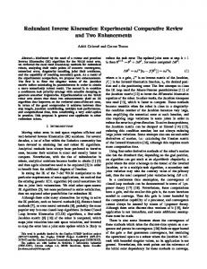
It is important to mention again that by using different αt ’s one can affect the path of the end-effector and the convergence time. Also, for a number of threads m large enough, the convergence should be quicker since in this case ~ k ’s will lie there will be a greater chance that one of the X t ~ right on top of the Xf inal . The pseudo-code of the proposed process is in Algorithm 2. In order to better understand our method, Figure 1 shows an analogy of the proposed algorithm for one dimension. The blue line represents the original Jacobian, while the red line would be one of the Jacobians found after adding white noise. For m = 2, the Jacobians Jt1 and Jt2 are created, leading to two possible solutions Q1t and Q2t . Through forward kinematics, each Qit determines a new pose Xti . In this simple example, Xt2 is selected since it is closer to the desired/final point Xf inal . In the next iteration t + 1, the process will continue from this position, Q2t .

Algorithm 2 : Proposed Parallel Algorithm ~ procedure IK(joints conf iguration : Q) n ← number of joints ~ t ← joints conf iguration Q 0 ~t ) ~ t = f (Q X 0 0 ~ ~ f inal k > εr do while kXt − X for each joint c ∈ [1 ... nQ ] do ~ ~ Jc = ∂X ∂qi = Xt − f (Qt + ∂qc ) end-for ~ t − f (Q ~ t + ∂qt ) Jt = X create m threads thread-do k ← thread ID Jtk = Jt + ℵ (0, ΣJ ) if n = 6 ~ kt = (Jtk )−1 ∗ αt (X ~ f inal − X ~ t) △Q else ~ f inal − X ~ t) ~ k = (J k )−P ∗ αt (X △Q t t end-if ~ t + △Q ~k ~k = Q Q t t k k ~ ~ Xt = f (Qt ) end-thread ~ f inal − X ~ k k is minimal} ~ t+1 = {X ~ k | kX X t t end-while end-procedure

Jacobian from section III-A. Our tests were performed on an Intel Xeon E5520 CPU running at 2.26 GHz. The typical speed-up obtained by the parallel approach was about two times of the single Jacobian, but in some cases, it reached 21 times, while keeping approximately the same error. A. Test for General Robot Manipulators TABLE I D-H PARAMETERS OF THE TESTED ROBOTS #

θ

d

a

α

#

θ

d

a

α

1

θ1

0

0

-90

1

θ1

700

750

-90

2

θ2

125.4

203.2

0

2

θ2

0

1250

0

3

θ3

0

-7.9

90

3

θ3

0

-55

-90

4

θ4

203.2

0

-90

4

θ4

1500

0

90

5

θ5

0

0

90

5

θ5

0

0

90

6

θ6

63.5

0

0

6

θ6

-230

0

180

(a) Puma 260 #

θ

d

a

α

1

θ1

0

0

-90

#

θ

d

a

2

θ2

149.09

431.8

0

1

θ1

0

250

0

3

θ3

0

-20.32

90

2

θ2

0

350

180

4

θ4

433.07

0

-90

3

0

d3

0

0

5

θ5

0

0

90

4

θ4

114.5

0

0

6

θ6

56.25

0

0

(c) Puma 560

Fig. 1.

Visual representation of the proposed method

IV. E XPERIMENTAL R ESULTS AND D ISCUSSION In this section, we present three experiments that were performed. For the first experiment, we ran our algorithm using four different non-redundant robots. In the second experiment, we selected several singular poses of the endeffector of a non-redundant robot as we moved the robot to/from those same poses. Finally, in the last experiment, we applied our method to a redundant 7 DoF robot presented in [2]. In average, the algorithm performed extremely well, returning a solution with sub-millimeter accuracy in under 20ms. For all cases below, in the third column of the tables, we report the number of iterations required by the parallel algorithm presented in section III-B versus the single inverse

(b) Kuka robot

α

(d) Scara robot

In this section, the cases for the inverse kinematics problem applied to four different robots are presented. Over 150 random final positions of the end-effector were used for test of a non-redundant Puma 260, Puma 560, Kuka and Scara robotic manipulators. The D-H parameters of the above mentioned robots can be found in Table I(a)-(d). All angles are in degree and all lengths in millimeters. It is important to point out that the initial position of the endeffector can affect the results as well as the path to the final position. Due to limitation of space, here we only report some of the most typical results and the total average. A spreadsheet with the remaining results can be found at http://vigir.missouri.edu/iros. Also, for the experiments reported here, the initial positions of the robots were set to the manufacturer-defined home position. The first three robots have six revolute joints, while the Scara robot has three revolute and one prismatic joints. The algorithm was implemented in C/C++ using POSIX threads. For the current implementation, the number m of threads used for each iteration was 16. As it can be seen in Tables II(a)-(d), in 12 of the 16 tests reported here, the algorithm was able to find the inverse kinematics solution in less than 20ms, which is considered “real time” for many applications. Again, the times shown below are typical for the tests not reported here. Also, the last rows of the tables list the average performance for all trials. The error column is the same for both the proposed method

TABLE II R ESULTS FOR TESTED ROBOTS End-effector position

Calculated joint configuration

# of iterations

Error

and orientation

(θ1 , θ2 , θ3 , θ4 , θ5 , θ6 )

(Proposed method /

Position / Orientation

time

Inverse Jacobian)

(mm) / (deg)

(ms)

(x, y, z, φr , φp , φy )

Execution

(-70, -160, 360, 30, 85, 0)

(158.74, -69.84, 41.48, -123.18, -112.69, 23.54)

28 / 764

0.97 / 0.36

18.627

(-350, 220, -130, 30, 45, -60)

(135.43, 40.96, 56.52, 52.10, -46.65, -97.70)

29 / 46

1.08 / 0.10

20.192

(-170, 100, 55, -25, 35, 10)

(5.89, -117.66, -30.60, 70.26, -171.14, -135.09)

25 / 40

0.82 / 0.44

19.790

(220, 300, 160, 45, -30, 30)

(39.41, -6.27, 72.10, 31.87, -92.32, 6.41)

19 / 33

1.00 / 0.58

14.387

28.50 / 169.5

0.85 / 0.46

22.811

Average of 34 tests

(a) Four arbitrarily chosen test cases and the average of all 34 trials for the Puma 260 End-effector position

Calculated joint configuration

# of iterations

Error

and orientation

(θ1 , θ2 , θ3 , θ4 , θ5 , θ6 )

(Proposed method /

Position / Orientation

time

Inverse Jacobian)

(mm) / (deg)

(ms)

(x, y, z, φr , φp , φy )

Execution

(-30, 500, 600, -89, -10, -75)

(-63.26, -110.13, 143.95, -59.48, -91.88, 129.90)

97 / 1976

0.84 / 0.49

66.276

(-300, 490, 420, -45, -30, 60)

(101.30, -9.75, 74.46, -120.66, -86.31, 116.04)

29 / 63

0.85 / 0.09

23.327

(400, 300, -1000, 88, 60, 80)

(26.52, 32.09, 13.26, -146.12, -44.21, -125.02)

28 / 102

0.77 / 1.64

22.056

(800, -720, 600, 30, -45, 60)

(-48.42, 112.80, 105.97, -54.26, -139.97, 171.98)

23 / 36

0.94 / 0.33

17.352

38.68 / 283.13

0.87 / 0.40

32.975

Average of 22 tests

(b) Four arbitrarily chosen test cases and the average of all 22 trials for the Kuka robot End-effector position

Calculated joint configuration

# of iterations

Error

and orientation

(θ1 , θ2 , θ3 , θ4 , θ5 , θ6 )

(Proposed method /

Position / Orientation

time

Inverse Jacobian)

(mm) / (deg)

(ms)

(x, y, z, φr , φp , φy )

Execution

(-200, -45, 870, -75, 25, -60)

(78.19, -105.66, 116.78, -45.96, -70.55, 52.69)

51 / 205

0.92 / 0.04

31.214

(-100, 150, 850, -45, 60, 0)

(-13.31, -87.73, 64.43, -27.54, 80.32, -12.14)

25 / 30

0.94 / 0.05

16.892

(450, 200, 200, 0, 60, -30)

(3.16, 35.74, -24.27, 34.15, 54.47, -23.28)

22 / 29

0.75 / 0.11

15.007

(150, 200, 250, 60, -45, 0)

(22.98, 27.91, -43.10, 49.70, -33.76, -16.43)

25 / 30

0.75 / 0.07

14.657

32.97 / 350.19

0.85 / 0.40

20.416

Average of 36 tests

(c) Four arbitrarily chosen test cases and the average of all 36 trials for the Puma 560 End-effector position

Calculated joint configuration

# of iterations

Error

and orientation

(θ1 , θ2 , d3 , θ4 )

(Proposed method /

Position / Orientation

time

Inverse Jacobian)

(mm) / (deg)

(ms)

(x, y, z, φr , φp , φy )

Execution

(500, 300, -150, -85, 0, 0)

(47.53, -28.28, 35.11, 103.34)

17 / 34

0.90 / 0.31

8.200

(350, 250, -135, 75, 0, 0)

(-19.09, 90.25, 20.49, -3.80)

30 / 36

0.91 / 0.01

12.088

(300, 500, -200, -85, 0, 0)

(42.47, 28.35, 85.40, 155.73)

26 / 37

0.89 / 0.03

11.039

(-350, 250, -135, -45, 0, 0)

(-161.01, -90.18, 20.49, 153.79)

29 / 34

0.73 / 0.01

12.313

24.45 / 221.65

0.8285 / 0.3285

8.931

Average of 20 tests

(d) Four arbitrarily chosen test cases and the average of all 20 trials for the Scara robot

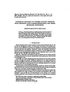
and the Inverse Jacobian since the termination conditions εr for both cases were set as shown. As Figure 2 indicates, in the majority of the trials, the end-effector moved in a smooth path directly towards the final position. However, due to the nature of the Inverse Kinematics functions which is not necessarily monotonic, some times the end effector moved in a wrong direction, which led to an increase in the number of iterations required for convergence. Figure 3 illustrates one such case that happened for the Puma 260 robot. B. Test for Robots at Singular Positions In this section, we report the results obtained for ten tests using the Puma 560. The results are presented in Table III. In some case (Table III(a)), the singularity was in the starting

positions, and for others (Table III(b)), the singularity was in the final positions. A total of six singular poses obtained from [19] were used in this section. The attentive reader will notice that the final joint configurations in Table III(b) do not always match the provided singular configuration, but yet, the final pose (x, y, z, roll, pitchandyaw) of the end-effector is the desired one. That is in fact a consequence of the very nature of a singular joint configuration, where the derivative of the motion is very flat (close to zero), leading to a close-toinfinite rate for its inverse. C. Test of a Redundant Robot Finally, we employed our algorithm for the redundant robot with 7 DoF in [2]. Table IV presents the results for

(a) X, Y and Z

(a) X, Y and Z

(b) roll, pitch and yaw

(b) roll, pitch and yaw

Fig. 2. Change in the end-effector pose versus the iteration number

Fig. 3. Change in the end-effector pose versus the iteration number

for an arbitrarily chosen test case

for an arbitrarily chosen test case

this test. As it can be seen in the Table IV, although the average number of iterations increased slightly with respect to the non-redundant cases, the algorithm still presents the same accuracy and robustness as in the non-redundant cases. V. C ONCLUSION AND F UTURE W ORK This paper presented a novel approach for the inverse kinematics problem for a general robotic manipulator. The method was implemented in parallel using C/C++ programming and POSIX threads. Unlike previous works which achieved an average of 5mm accuracy and 42ms execution time, our experimental results carried out on different robots showed that the proposed approach is able to find a solution with less than 1mm accuracy and in real time (20.48ms in average). The algorithm was validated using five robots, at singular and non-singular configurations, including a redundant robot. Many aspects of the algorithm can be further investigated. For example, the use of constraints, as to avoid obstacles, ˆ~ when selecting the best X towards the final position of the end-effector. Also, further investigation on the effect of αt both on the convergence of the algorithm and the accuracy of the final solution will be carried out. R EFERENCES [1] R. K¨oKer, “A genetic algorithm approach to a neural-network-based inverse kinematics solution of robotic manipulators based on error minimization,” Inf. Sci., vol. 222, pp. 528–543, Feb. 2013. [Online]. Available: http://dx.doi.org/10.1016/j.ins.2012.07.051

[2] O. Ivlev and A. Graser, “Resolving redundancy of series kinematic chains through imaginary links,” in in Proc. CESA 98 IMACS Multiconference. Computational Engineering in Systems Applications, 1998, pp. 477–482. [3] O. A. Aguilar and J. C. Huegel, “Inverse kinematics solution for robotic manipulators using a cuda-based parallel genetic algorithm,” in Proceedings of the 10th Mexican international conference on Advances in Artificial Intelligence - Volume Part I, ser. MICAI’11. Berlin, Heidelberg: Springer-Verlag, 2011, pp. 490–503. [4] D. Pham, M. Castellani, and A. Fahmy, “Learning the inverse kinematics of a robot manipulator using the bees algorithm,” in Industrial Informatics, 2008. INDIN 2008. 6th IEEE International Conference on, july 2008, pp. 493–498. [5] Q. Z. Liao and Q. Z. C. G. Liang, “A novel approach to the displacement analysis of general spatial 7r mechanism,” Chinese Journal of Mechanical Engineering, vol. 22, no. 3, pp. 1–9, 1986. [6] H.-Y. Lee and C.-G. Liang, “Displacement analysis of the spatial 7-link 6r-p linkages,” Mechanism and Machine Theory, vol. 22, no. 1, pp. 1 – 11, 1987. [Online]. Available: http://www.sciencedirect.com/science/article/pii/0094114X8790070X [7] M. Raghavan and B. Roth, “Inverse kinematics of the general 6R manipulator and related linkages,” Journal of Mechanical Design, vol. 115, no. 3, pp. 502–508, 1993. [Online]. Available: http://dx.doi.org/10.1115/1.2919218 [8] D. Manocha. and J. F. Canny, “Real time inverse kinematics for general 6r manipulators,” in Robotics and Automation, 1992. Proceedings., 1992 IEEE International Conference on. IEEE, 1992, pp. 383–389. [9] D. Manocha and J. F. Canny, “Efficient inverse kinematics for general 6r manipulators,” Robotics and Automation, IEEE Transactions on, vol. 10, no. 5, pp. 648–657, 1994. [10] D. Demers and K. Kreutz-Delgado, Inverse Kinematics of Dextrous Manipulators. 525 B Street, Suite 1900, San Diego, CA 92101-4495, USA: Academic Press, 1997, ch. 4.2, pp. 77–80. [11] S. Kumar, N. Sukavanam, and R. Balasubramanian, “An optimization approach to solve the inverse kinematics of redundant manipulator,” International Joural of Information and Systems Sciences, vol. 6, no. 4, pp. 414–423, 2010.

TABLE III R ESULTS FOR P UMA 560 IN SINGULAR POSITIONS End-effector position

Calculated joint configuration

# of iterations

Error

and orientation

(θ1 , θ2 , θ3 , θ4 , θ5 , θ6 )

(Proposed method /

Position / Orientation

time

Inverse Jacobian)

(mm) / (deg)

(ms)

(x, y, z, φr , φp , φy ) Initial position: (θ1 = 90,

θ2 = −90,

θ3 = 92.6864,

θ4 = 0,

θ5 = 90,

Execution

θ6 = 0)

(-100, 150, 850, 30, 60, 0)

(86.74, -98.57, 125.95, -74.97, 48.15, 30.73)

30 / 325

0.91 / 0.21

21.152

(-200, -45, 870, -75, 25, -60)

(78.84, -105.72, 117.15, 133.85, 70.78, -127.40)

46 / 182

0.76 / 0.21

29.711

(-300, 400, -200, 75, -60, 75)

(-39.87, -149.38, -18.62, -37.67, 87.94, -143.26)

26 / 871

1.16 / 0.18

17.546

(-200, 200, 150, 45, 30, -60)

(-20.59, -82.16, -40.53, 37.90, -99.91, 91.39)

16 / 35

0.92 / 1.42

12.614

Initial position: (θ1 = 90,

θ2 = −45,

θ3 = 2.9167,

θ4 = 0,

θ5 = 90,

θ6 = 0)

(-55, 205, 750, 10, -15, 30)

(62.95, -42.07, 26.75, 22.37, -18.63, -72.23)

26 / 127

0.91 / 0.02

23.486

(280, 330, 170, -90, 0, 15)

(28.50, 44.76, -27.58, -12.57, -30.56, -105.54)

26 / 37

0.69 / 0.38

18.383

(a) Singular initial position End-effector position

Calculated joint configuration

# of iterations

Error

and orientation (x, y, z, φr , φp , φy )

(θ1 , θ2 , θ3 , θ4 , θ5 , θ6 )

(Proposed method /

Position / Orientation

time

Inverse Jacobian)

(mm) / (deg)

(ms)

(32.99, -44.19, 2.80, -83.23, -2.15, 81.03)

32 / 50

0.78 / 0.21

20.035

(-27.52, -43.65, 2.86, -0.42, 43.66, -5.01)

26 / 42

0.81 / 0.03

17.593

(14.45, -87.69, 88.58, -178.59, 2.78, 89.18)

29 / 66

0.90 / 0.29

19.030

(77.16, -88.39, 87.89, 4.51, 63.00, -0.09)

28 / 54

0.80 / 0.32

21.494

/ Joint configuration (θ1 , θ2 , θ3 , θ4 , θ5 , θ6 ) (-107.19, 110.27, 654.87, 30, -42.08, 0)

Execution

/ (30, -45, 2.9167, 0, 0, 0) (77.02, 127.68, 669.30, -30, 2.92, 0) / (-30, -45, 2.9167, 0 ,45 ,0) (-36.04, 144.69, 921.53, -75, 0, 2.69) / (15, -90, 92.6864, 30, 0, 60) (-138.14, 75.11, 891.16, 80, 62.69, 0) / (80, -90, 92.6864, 0, 60, 0)

(b) Singular final position TABLE IV R ESULTS FOR 7-D O F REDUNDANT ROBOT IN [2] End-effector position

Calculated joint configuration

# of iterations

Error

and orientation

(θ1 , θ2 , θ3 , θ4 , θ5 , θ6 , θ7 )

(Proposed method /

Position / Orientation

time

Inverse Jacobian)

(mm) / (deg)

(ms)

(x, y, z, φr , φp , φy )

Execution

(1000, -600, 200, 60, 0, 75)

(-20.39, 83.17, 86.43, -22.11, -59.30, 25.65, -121.27)

31 / 110

0.92 / 0.43

14.215

(0, 0, 1400, -30, 0, 0)

(-113.77, 0.46, 12.52, -1.36, 8.06, 1.39, 63.11)

29 / 215

0.75 / 0.25

13.467

(-50, -30, 1000, 30, 60, -45)

(-110.26, 45.44, -7.52, -26.61, 15.47, -88.65, 157.77)

44 / 123

0.76 / 0.26

19.490

(800, 400, 550, -10, 60, 30)

(-119.56, -103.63, 45.52, 90.60, 4.12, -38.34, -67.52)

72 / 124

0.90 / 0.39

29.621

39.33 / 95.14

0.85 / 0.41

14.749

Average of 21 tests

[12] P. Kalra, P. Mahapatra, and D. Aggarwal, “An evolutionary approach for solving the multimodal inverse kinematics problem of industrial robots,” Mechanism and Machine Theory, vol. 41, no. 10, pp. 1213 – 1229, 2006. [Online]. Available: http://www.sciencedirect.com/science/article/pii/S0094114X05002053 [13] A. T. Hasan, N. Ismail, A. M. S. Hamouda, I. Aris, M. H. Marhaban, and H. M. A. A. Al-Assadi, “Artificial neural networkbased kinematics jacobian solution for serial manipulator passing through singular configurations,” Advances Engineering Software., vol. 41, no. 2, pp. 359–367, Feb. 2010. [Online]. Available: http://dx.doi.org/10.1016/j.advengsoft.2009.06.006 [14] S. Qiao, Q. Liao, S. Wei, and H.-J. Su, “Inverse kinematic analysis of the general 6r serial manipulators based on double quaternions,” Mechanism and Machine Theory, vol. 45, no. 2, pp. 193 – 199, 2010. [Online]. Available: http://www.sciencedirect.com/science/article/pii/S0094114X09001098 [15] M. Husty, M. Pfurner, and H.-P. Schrocker, “A new and efficient algorithm for the inverse kinematics of a general serial 6r manipulator,” Mechanism and Machine Theory, vol. 42, no. 1, pp. 66–81, 2007. [16] A. Escande, N. Mansard, and P. B. Wieber, “Fast resolution of hierarchized inverse kinematics with inequality constraints,” in Robotics and Automation (ICRA), 2010 IEEE International Conference on, 2010, pp.

3733–3738. [17] O. Kanoun, “Real-time prioritized kinematic control under inequality constraints for redundant manipulators,” in Proceedings of Robotics: Science and Systems, Los Angeles, CA, USA, June 2011. [18] J. Parker, A. Khoogar, and D. Goldberg, “Inverse kinematics of redundant robots using genetic algorithms,” in Robotics and Automation, 1989. Proceedings., 1989 IEEE International Conference on, may 1989, pp. 271 –276 vol.1. [19] F.-T. Cheng, T.-L. Hour, Y.-Y. Sun, and T.-H. Chen, “Study and resolution of singularities for a 6-dof puma manipulator,” Trans. Sys. Man Cyber. Part B, vol. 27, no. 2, pp. 332–343, Apr. 1997. [Online]. Available: http://dx.doi.org/10.1109/3477.558842