W3C's DOM API [5] manifests this model. Basically there are four kinds of node in a data tree: a document node for the document itself which is the root for the.
From Tree Patterns to Generalized Tree Patterns: On Efficient Evaluation of XQuery by Zhimin Chen B.S., Zhongshan University, China, 1994
A THESIS SUBMITTED IN PARTIAL FULFILLMENT OF THE REQUIREMENTS FOR THE DEGREE OF
Master of Science in THE FACULTY OF GRADUATE STUDIES (Department of Computer Science)
we accept this thesis as conforming to the required standard
The University of British Columbia August 2003 c Zhimin Chen, 2003
Abstract XQuery is the de facto standard XML query language, and it is important to have efficient query evaluation techniques available for it. It is a well-known fact that a formal bulk algebra is essential for efficient query evaluation, and the Tree Algebra for XML (TAX), among others, is invented for this purpose. It can be shown in this thesis that a substantial subset of XQuery can be expressed as TAX. An XML document is often modelled as an ordered label tree. A core operation in the evaluation of XQuery is the finding of matches for specified tree patterns against the data tree (or forest), and there has been much work towards algorithms for finding such matches efficiently. Multiple XPath expressions can be evaluated by computing one or more tree pattern matches. However, because of the flexibility of XML data, the efficient evaluation of XQuery queries as a whole is much more than a tree pattern match and combining matchings of multiple tree patterns is not the most efficient evaluation plan for XQuery. In this thesis a structure called generalized tree pattern (GTP) is proposed to concisely represent a whole XQuery expression. Evaluating a query reduces to finding the matches of its GTP, which leads to more efficient evaluation plans. Algorithms are developed to translate an XQuery expression, possibly involving join, quantifiers, grouping, aggregation and nesting, to its GTP, and to generate
ii
efficient physical plans for a specified GTP. XML data often conforms to a schema. Relevant constraints from the schema give rise to further opportunities to optimize queries. Algorithms are given in the thesis to automatically infer structural constraints from a given schema and to simplify a GTP given a set of structural constraints. Finally, a detailed set of experiments using the TIMBER XML database system shows that plans via GTPs (with or without schema knowledge) significantly outperform plans based on navigation and straightforward plans obtained directly from the query.
iii
Contents Abstract
ii
Contents
iv
List of Figures
vii
Acknowledgments
ix
Dedication
x
1 Introduction
1
1.1
XML . . . . . . . . . . . . . . . . . . . . . . . . . . . . . . . . . . . .
1
1.2
Tree Pattern Query . . . . . . . . . . . . . . . . . . . . . . . . . . . .
2
1.3
XQuery . . . . . . . . . . . . . . . . . . . . . . . . . . . . . . . . . .
3
1.4
Challenges In Translating XQuery Into TPQs . . . . . . . . . . . . .
4
1.5
Generalized Tree Pattern . . . . . . . . . . . . . . . . . . . . . . . .
5
1.6
Problem Statement and Contributions . . . . . . . . . . . . . . . . .
6
1.7
Related Work . . . . . . . . . . . . . . . . . . . . . . . . . . . . . . .
7
1.8
Chapters Overview . . . . . . . . . . . . . . . . . . . . . . . . . . . .
8
iv
2 Background 2.1
2.2
10
Tree Algebra For XML . . . . . . . . . . . . . . . . . . . . . . . . . .
10
2.1.1
Basic TAX Operators . . . . . . . . . . . . . . . . . . . . . .
11
Physical Algebra . . . . . . . . . . . . . . . . . . . . . . . . . . . . .
13
2.2.1
13
Physical Operators . . . . . . . . . . . . . . . . . . . . . . . .
3 TAX Translation For XQuery
16
3.1
Grammar For XQuery Fragment . . . . . . . . . . . . . . . . . . . .
16
3.2
Normalization . . . . . . . . . . . . . . . . . . . . . . . . . . . . . . .
17
3.2.1
XQuery in Canonical Form . . . . . . . . . . . . . . . . . . .
17
3.2.2
XQuery Normalization . . . . . . . . . . . . . . . . . . . . . .
18
3.3
Derived TAX Operators . . . . . . . . . . . . . . . . . . . . . . . . .
23
3.4
Translation . . . . . . . . . . . . . . . . . . . . . . . . . . . . . . . .
24
3.4.1
24
Single Block XQuery Translation . . . . . . . . . . . . . . . .
4 Generalized Tree Patterns
38
4.1
Basic GTPs . . . . . . . . . . . . . . . . . . . . . . . . . . . . . . . .
38
4.2
Join Queries . . . . . . . . . . . . . . . . . . . . . . . . . . . . . . . .
41
4.3
Grouping, Aggregation, and Quantifiers . . . . . . . . . . . . . . . .
42
4.4
Nested Queries . . . . . . . . . . . . . . . . . . . . . . . . . . . . . .
45
4.5
Translating XQuery to GTP . . . . . . . . . . . . . . . . . . . . . . .
47
4.6
Translating GTP Into an Evaluation Plan . . . . . . . . . . . . . . .
49
5 Schema-Aware Optimization 5.1
57
Logical Optimization . . . . . . . . . . . . . . . . . . . . . . . . . . .
57
5.1.1
Avoidance Constraint and Internal node elimination . . . . .
58
5.1.2
Identified Constraint and Identifying Nodes With the Same Tag 58 v
5.1.3
Leaf elimination and Emptiness detection . . . . . . . . . . .
59
5.1.4
GTP Simplification . . . . . . . . . . . . . . . . . . . . . . . .
59
5.2
Physical Optimization . . . . . . . . . . . . . . . . . . . . . . . . . .
64
5.3
Constraint Inference . . . . . . . . . . . . . . . . . . . . . . . . . . .
66
5.3.1
Regular Tree Grammar . . . . . . . . . . . . . . . . . . . . .
66
5.3.2
Inferring Avoidance Constraints
. . . . . . . . . . . . . . . .
66
5.3.3
Inferring Quantifier Constraints . . . . . . . . . . . . . . . . .
67
6 Experiment
72
6.1
Experiment Setting . . . . . . . . . . . . . . . . . . . . . . . . . . . .
72
6.2
GTP Plans and TAX Plans . . . . . . . . . . . . . . . . . . . . . . .
73
6.3
Scalability . . . . . . . . . . . . . . . . . . . . . . . . . . . . . . . . .
75
6.4
Schema-Aware Optimization . . . . . . . . . . . . . . . . . . . . . . .
76
7 Conclusion and Future Work
77
Bibliography
79
vi
List of Figures 1.1
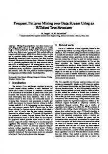
Two Example Tree Pattern Queries: (a) P 1 and (b) P4 . Single (double) edge represents parent-child (ancestor-descendant) relationship.
1.2
2
An Example XQuery query and corresponding Generalized Tree Pattern Query. Solid (dotted) edges = compulsory (optional) relationship. Group numbers of nodes in parentheses. . . . . . . . . . . . . .
6
3.1
Grammar for XQuery Fragment. . . . . . . . . . . . . . . . . . . . .
16
3.2
Example of normalization. Qa is an example query, Qb is the result after applying Lemma 3.1 to Qa to remove filters, Qc is the result after applying Lemma 3.2 to Qb, and Qd is the result of applying Lemma 3.3 to Qc.
. . . . . . . . . . . . . . . . . . . . . . . . . . .
21
3.3
An example query and the translated TAX expression. . . . . . . . .
35
3.4
An example disjunctive query and the translated TAX expression. .
36
3.5
An example nested query and the translated TAX expression. . . . .
37
4.1
Extension to handle ‘undefined’ truth value. . . . . . . . . . . . . . .
39
4.2
(a) Sample XML data. (b) Pattern matches of GTP of Fig. 1.2(b). The numbers in (b) are the startPoss of the nodes in (a) numbered in the interval encoding scheme [2]. . . . . . . . . . . . . . . . . . . . vii
40
4.3
A query involving join and corresponding GTP. . . . . . . . . . . . .
42
4.4
An example universal query and corresponding universal GTP. . . .
44
4.5
An Example query with nesting & join and corresponding GTP. . .
45
4.6
Algorithm GTP . . . . . . . . . . . . . . . . . . . . . . . . . . . . . .
48
4.7
Physical Plan from the GTP of Figure 1.2(b). . . . . . . . . . . . .
52
4.8
Physical Plan from the GTP of Figure 4.5(b). . . . . . . . . . . . .
54
4.9
Algorithm planGen . . . . . . . . . . . . . . . . . . . . . . . . . . . .
56
5.1
Algorithm pruneGTP . . . . . . . . . . . . . . . . . . . . . . . . . . .
60
5.2
A sample XQuery query, the associated GTP, and the simplified GTP 61
5.3
Algorithm c-occurrences . . . . . . . . . . . . . . . . . . . . . . . .
68
5.4
Algorithm d-occurrences . . . . . . . . . . . . . . . . . . . . . . . .
71
6.1
Queries Qa, Qb, Qc
73
6.2
CPU timings (secs) for XMark factor 1. Algorithms used: BASE =
. . . . . . . . . . . . . . . . . . . . . . . . . . .
Baseline plan, GTP = GTP plan, SCH = GTP with schema optimization. The queries are XMark queries (XM5, XM20, . . . ) and the queries (Qa, Qb, Qc) seen in Figure 6.1. . . . . . . . . . . . . . . . . 6.3
CPU timings (secs). Using GTP with no schema-aware optimization or value index. . . . . . . . . . . . . . . . . . . . . . . . . . . . . . .
6.4
74
75
CPU timings (Comparison of GTP and GTP with schema optimization plans for XM5, Qa and XM20. . . . . . . . . . . . . . . . . . . .
viii
76
Acknowledgments This thesis would not have been possible without the helps from many people. First and foremost, I am very grateful to Dr. Laks V.S. Lakshmanan, my supervisor, for his great guidance and support throughout this thesis work. I would also like to thank Dr. Raymond T. Ng and Dr. Anne Condon for being in my thesis committee and for their valuable advices and comments. Other thanks are due to Dr. George Tsiknis for reviewing my thesis and providing much advice and feedback. I have had the pleasure of working with all members of the database lab over the years, and owe a lot of thanks for their help and suggestion. Last but not the least, I owe a great deal of thanks to the TIMBER research group in University of Michigan, especially to Dr. H.V. Jagadish and Stelios Paparizos, for all their help in this thesis work. In particular, the experimental results reported in this thesis was conducted on the TIMBER system at University of Michigan by Stelios Paparizos.
Zhimin Chen
The University of British Columbia August 2003
ix
To my parents
x
Chapter 1
Introduction 1.1
XML
XML [4] is the de facto standard format for data exchange. Syntactically, a wellformed XML document is often modelled as a labelled rooted ordered tree. The W3C’s DOM API [5] manifests this model. Basically there are four kinds of node in a data tree: a document node for the document itself which is the root for the data tree, an element node for every element in the document, an attribute node for every attribute specified in every element, and text nodes which can be viewed as the values of elements. Some attributes (for instance the IDREF attributes) may have special semantics of acting as hyperlinks within a tree or even crossing the trees, and therefore the semantic data model of an XML document may become a rooted directed graph. Nevertheless, in a formal query algebra such as TAX, these attributes are treated just like other common attributes. A query involving navigation along the IDREF links can be expressed as predicates constrained on the value of the ID and IDREF attributes, though the implementation may choose some
1
$p
$s
$p.tag = person & $s.tag = state & $l.tag = profile & $g.tag = age & $g.content > 25 & $s.content != ‘MI’
$l $g (a)
$p $p.tag = person & $w.tag = watches & $t.tag = watch
$w $t (b)
Figure 1.1: Two Example Tree Pattern Queries: (a) P 1 and (b) P4 . Single (double) edge represents parent-child (ancestor-descendant) relationship. special data structure (join index, for instance) to speed up the evaluation of such predicates. Thus, conceptually this labelled-rooted-ordered-tree data model can be used without loss of generality, and is adopted within this thesis.
1.2
Tree Pattern Query
With the rapid adoption of XML as an alternative data model, querying XML data attracts considerable research efforts. In most proposed XML query languages, including XQuery [8], which is considered as the de facto standard of XML query language, query is performed by binding variables to the data nodes of interest. The abstraction for specifying the bindings between variables and data nodes is the so-called tree pattern (query) (TP(Q)), which is a tree T with nodes labelled by variables, together with a boolean formula F specifying constraints on the nodes and their properties, including their tags, attributes, and contents. The tree consists of two kinds of edges – parent-child (pc) and ancestor-descendant (ad) edges. Figure 1.1(a)-(b) shows example TPQs; in (b), we call node $w an ad-child of $p, and a pc-parent of $t. 2
The semantics of a TPQ P = (T, F ) is captured by the notion of a pattern match – a mapping from the pattern nodes to nodes in an XML database such that the formula associated with the pattern as well as the structural relationships among pattern nodes is satisfied. The TPQ in Figure 1.1(a) (if applied to the auction.xml document of the XMark benchmark [29]) matches person nodes that have a state subelement with value 6= ‘MI’ and a profile with age > 25. The state node may be any descendant of the person node. Viewed as a query, the answer to a TPQ is the set of all node bindings corresponding to valid matches. The central importance of TPQs to XML query evaluation is evident from the flurry of recent research on efficient evaluation of TPQs [31, 2, 11].
1.3
XQuery
XQuery [8] is the recommended query language by W3C to retrieve information from many types of XML data sources, whether they store data physically in XML or expose a view as XML via middleware. One characteristic in the data model of XQuery is that every expression is evaluated to a sequence. The order of the sequence is by default the one obtained by a depth first traversal of the document, or a user-defined order specified in an OrderBy clause. The basic construct of XQuery expression is the so-called FLWOR expression. The semantics of the FLWOR expression can be informally illustrated by a simple query against the auction.xml document from the XMark project [29] shown in Figure 1.2(a). The for clause generates a sequence of person elements and binds $p to each element in turn, and then for each binding of $p, binds $l to each child profile element in turn. The result of the for clause is a stream of pairs of 3
bindings of $p and $l. The where clause filters the stream by retaining only the pairs which represent a person who is not living in the Michigan state and is older than 25. The return clause constructs a new result element for each surviving pair, which contains a sequence of watches elements and a sequence of interest elements generated from the bindings in that pair. The result of the whole FLWOR expression is a sequence generated by concatenating all the newly constructed result elements. The let clause binds a variable to all elements in a sequence as a whole. In contrast, the for clause binds a variable to each element in a sequence by iterating the sequence in turn. The optional OrderBy clause orders the surviving tuples of bindings generated by the for and let clause according to some criteria specified by the user.
1.4
Challenges In Translating XQuery Into TPQs
While XQuery expression evaluation includes the matching of tree patterns, and hence can include TPQ evaluation as a component, there is much more to XQuery than simply TPQ. In particular, the possibility of quantification in conditions (e.g., EVERY), the possibility of optional elements in a return clause, and the many different forms of return results that can be constructed using just slightly differing XQuery expressions, all involve much more than merely obtaining variable bindings from a TPQ evaluation. Combining query results from multiple TPQs to answer an XQuery query results in extra pattern matchings and extra joins which are not necessary. Although a smart optimizer can possibly eliminate these unnecessary pattern matchings and joins, it is unclear how to do it in a complete and systematic way.
4
1.5
Generalized Tree Pattern
To facilitate an efficient evaluation of XQuery queries, the notion of generalized tree pattern (GTP) is proposed in this thesis work. Intuitively, a GTP provides an abstraction of the work that needs to be done toward query evaluation, and provides clues for doing this work while making as few passes over the input data as possible. As a preview, Figure 1.2(b) shows a sample query (against the auction.xml document of the XMark benchmark [29]) as well as the associated (rather simple in this case) GTP. The GTP has solid and dotted edges. Solid edges represent mandatory relationships (pc or ad) just like edges of a TPQ. Dotted edges denote optional relationships: e.g., $i optionally may be a child of $l, and $w optionally may be a descendant of $p. The GTP can be informally understood as follows: (1) Find matches for all nodes connected to the root by only solid edges. (2) Next, find matches to the remaining nodes (whose path to the GTP root involves one or more dotted edges), if they exist. We will show later that this semantics of GTPs is a key feature enabling them to be used as a basic data structure with which to obtain all valid bindings necessary to answer an XQuery query. In particular, GTP can be used to answer a complex query involving quantifiers, grouping, aggregation, and nesting. In the experimental study section (Chapter 6), we will compare plans from translating XQuery into GTP and then into physical algebraic expressions with the plans from translating XQuery into a sequel of TPQs and then into physical algebra. We will show that the GTP plans always far outperform the TPQ plans, by an order of magnitude in most cases. We will also demonstrate the savings obtained by incorporation of schema knowledge into the GTP plans in query optimization.
5
FOR $p IN document("auction.xml")//person, $l IN $p/profile WHERE $l/age > 25 AND $p/state != ‘MI’ RETURN {$p//watches/watch}{$l/interest} (a)
$p (0) (0) $s $w (1) (1) $t
(0) $l
$p.tag = person & $s.tag = state & $l.tag = profile & $i.tag = interest & $w.tag = watches & $t.tag = watch & $g.tag = age & $g.content > 25 & $s.content != ‘MI’
$g (0) $i (2) (b)
Figure 1.2: An Example XQuery query and corresponding Generalized Tree Pattern Query. Solid (dotted) edges = compulsory (optional) relationship. Group numbers of nodes in parentheses.
1.6
Problem Statement and Contributions
This thesis aims at the problem of XQuery evaluation in the setting of native XML DBMS: Given a (restricted) FLWR expression, our method will translate it into an evaluation plan expressed in a physical algebra typically available in a native XML DBMS, and optimize the plan with or without schema knowledge. The main contributions of this thesis include the following: • Show that an XQuery FLWR expression can be translated into a sequel of TPQs expressed in a formal bulk algebra for XML (Chapter 3) • Propose the notion of generalized tree pattern (Chapter 4) • Give an algorithm for translating an XQuery FLWR expression into a GTP (Chapter 4) 6
• Give an algorithm that translates a GTP into an equivalent plan in the physical algebra used in TIMBER, a native XML database (Chapter 4) • Show how schema knowledge can be exploited to remove redundant parts of the GTP, and to eliminate unnecessary operators in the physical query plan (Chapter 5) • Give algorithms to extract the relevant knowledge from a DTD (Chapter 5)
1.7
Related Work
There are three major approaches to XML data management and query evaluation: the navigation-based, the relational, and the native approach. Galax [24] is a well-known example of a navigation-based XQuery query processing system. The major issue of the navigational approach is that it results in an implementation as evaluating a query as a series of nested loops, whereas a more efficient evaluation plan is frequently possible. Relational approaches to XQuery implementation include [13, 25, 10, 30, 23], while [3] uses an object-relational approach. The core of the relational approach is to map XML data to relational schemas and to translate the queries into SQL. Because of the mismatch of the rich structure of the XML data model and the rigid tabular relational data model, the translated SQL queries usually are complex correlated queries involving many joins and even more expensive recursions. Most of the relational implementations have focused on a restrictive subset of XQuery, with the exception of the ”dynamic intervals” paper [10], in which algorithms were given to translate a broader subset of XQuery, similar to that used in this thesis work, into SQL. 7
Some examples of native approaches to XML query processing include Natix [12], Tamino [22], and TIMBER [16]. Most previous work on native XQuery implementation has focused on efficient physical placement of XML data at the page level [12], efficient evaluation of XPath expressions via structural join [2] and holistic join [11], and optimal ordering of structural joins for pattern matching [14]. TIMBER [16] makes extensive use of structural joins for pattern match, as does the Niagara system [21]. We are not aware of any papers focusing on optimization and plan generation for XQuery queries as a whole for native systems. Recently, there has been much interest in optimizing (fragments of) XPath expressions by reasoning with TPQs or irs variants, possibly making use of any available schema knowledge [32, 19, 28]. GTPs enable similar logical optimization to be performed for XQueries as a whole, with or without schema knowledge. Secondly, previous work on schema-aware optimization for XML queries (e.g., [28]) only focused on XPath fragments. In this thesis we have developed the initial ideas for a similar exercise for XQuery and reported results from our experiments suggesting when schema-based optimization can (not) be expected to pay off big time. We are not aware of similar results from previous work.
1.8
Chapters Overview
The remainder of this thesis is organized as follows. Chapter 2 reviews the Tree Algebra for XML (TAX) and the physical operators in the TIMBER system. Chapter 3 discusses the algorithm to translate XQuery into TAX. Chapter 4 develops GTP for variant constructs of XQuery. Chapter 5 discusses logical and physical optimizations by applying schema knowledge to GTP, and gives algorithm to extract relevant schema information for optimization from DTD. Chapter 6 focuses 8
on the experimental studies of the performance of evaluation plan and the optimizations facilitated by GTP. Chapter 7 summarizes the thesis work and discuss future extension to GTP.
9
Chapter 2
Background 2.1
Tree Algebra For XML
It is a long established fact that a formal bulk algebra which processes data in a setat-a-time fashion is essential to efficient processing on large databases. The algebra for XQuery proposed by the W3C XQuery working group [9], though is useful in investigating the formal semantics of XQuery, yet appears unlikely to form the basis of efficient evaluation of XQuery because of its lack of set-at-a-time processing capability. Consequently, we choose the Tree Algebra for XML (TAX) [15] as the basis to study query translation and optimization for XQuery in this thesis work. TAX is a bulk algebra similar to relational algebra augmented with aggregation, except that each TAX operator manipulates sets of ordered labelled trees instead of set of tuples. Two concepts in TAX, namely pattern tree and witness tree, are key to manipulating trees. Their formal definitions [15] are given as follows. Definition 2.1 (Pattern Tree). A pattern tree is a pair P = (T, F ) where T = (V, E) is a node-labelled and edge-labelled tree and F is a boolean formula such
10
that: (i) each node in V is labelled by a distinct integer; (ii) each edge in E is labelled either as pc (for parent-child) or ad (ancestor-descendent); and (iii) F is a boolean combination of predicates applicable to nodes. Definition 2.2 (Embedding). Let P = (T , F) be a pattern and C a collection of trees. An embedding of P into C is a total mapping h : V → C from the nodes of P such that: (i) h preserves the structural relationships in P, i.e., whenever h is defined on nodes u, v and there is a pc (ad) edge (u, v) in G, then h(v) is a child (descendant) of h(u); and (ii) the image of h satisfies the boolean formula F . Each embedding induces a witness tree by retaining only the nodes in the embedding and restricting the original tree structure to the retained nodes. Multiple ways of embedding a pattern into a data tree results in multiple witness tree, one per each embedding. TAX operators are defined on top of the concepts of pattern tree and witness tree.
2.1.1
Basic TAX Operators
Selection. Selection σP,SL takes a collection of trees C as input and produces a collection of trees as output. Each tree in the output collection is a witness tree induced by some embedding of P into C, except that if a pattern node $x appears in SL, the whole subtree rooted at the node which witnesses $x is returned as the output. Projection. Projection πP,P L takes a pattern P and a projection list P L as its parameters, where P L is a list of pattern nodes in P , possibly adorned with ”*”. Given a collection of trees C as input, projection π P,P L retains a node in the output if it witnesses a pattern node in P L under some embedding of P into C, or if it is the descendant of a node which witnesses a pattern node adorned with ”*” in P L. 11
Product. Product takes two collections of trees C and D as input. For each pair Ti ∈ C and Tj ∈ D, the output of C × D contains a tree, whose root is a new node with a tag name of tax prod root and with T i as its left subtree and Tj as its right subtree. Join is expressed as product followed by selection; projection join is expressed as product followed by projection. Grouping. The groupby operator γP,gb,ol takes a pattern tree, a groupby basis and an order list as its parameters. The groupby operator partitions all the witness trees obtained from embedding P into C into groups, where all the witness trees in the same group have the same value on the nodes witnessed a node appearing in gb. For each group, a tree is output as follows. The tree has a root, which has a tag tax group root and two children. The left child has a tag tax group basis, and a subtree for the groupby basis. The right child has a tag tax group subroot, and its children are the source trees in C for the witness tree in the group, ordered according to the order list. The duplicate elimination operator δ P,DL (where P is a pattern tree and DL is a list of pattern nodes) can be derived from the groupby operator [15] by applying γP,DL,ol , where ol is any order list, to the input collection C and keeping only one tree per partition. Aggregation. The aggregation operator takes a pattern tree P , an aggregate function f , and a update specification as its parameters. The update specification denotes where to insert the new node representing the aggregation value. For instance, an aggregation operator with an update specification afterlastchild($i) results in a new node with attribute-value pairs {,} inserted as the rightmost child of the witness node for $i.
12
2.2
Physical Algebra
The native XML database TIMBER [16] develops a physical algebra [18] complete with respect to TAX. A query is eventually translated into a physical plan in the format of a directed acyclic graph (DAG) of physical operators. The engine then executes the physical plan to produce query result.
2.2.1
Physical Operators
Index Scan. The index scan operator IS p (S) takes a predicate p as its parameter. For each input tree in S, output each node satisfying p using an index. Filter. The filter operator Fp (S) takes a predicate p as its parameter. Given a sequence of trees S, it outputs only the trees satisfying the filter predicate p. The order in the input sequence is preserved in the output. Sort. Given a sequence of trees S, the sort operator S b (S) sort S according to the sorting basis b. The order of the output sequence reflects the sorting procedure (e.g., by value or by node id order of specified node). Value Join. The value join operator J p (S1 , S2 ) takes two sequences of trees as input and a join predicate as its parameter. It joins S 1 and S2 based on a valuebased comparison (in contrast to the structural join operator below) via the join predicate p. The order of the output sequence reflects that of S 1 . A sort-merge join algorithm similar to that used in the relational DBMS is used, except that an extra sorting procedure is included to resort the output of the sort-merge join to conform to the left S1 input sequence order. As in the relational world, the physical algebra includes the left-outer value join as a variant with its standard meaning: each tree in S1 will be returned in the output sequence even if there is no match with a tree in S2 . 13
Structural Join. The structural join operator SJ r (S1 , S2 ) takes two sequences of trees, S1 and S2 , as input. Both S1 and S2 must be sorted based on the node id of the desired structural relationship. The operator joins S 1 and S2 based on the structural relationship r (ad or pc) between them for each pair. The output is sorted by S 1 or S2 as needed. Variants include: the Outer Structural Join (OSJ) where all of S 1 is included in the output, Semi Structural Join (SSJ) [1] where only S 1 is retained in the output, Structural Anti-Join (ASJ) where the two inputs are joined based on one not being the ad/pc-relative of the other, and combinations. Interval encoding is key to the underlying algorithm of the structural join operator [2]. Each node is assigned a pair (startP os, endP os) such that the followings hold for each pair of nodes m and n: startP osm < startP osn if m precedes n in document order; the interval [startP osm , endP osm ] contains [startP osn , endP osn ] if m is an ancestor of n, or their intervals are disjoined if there is no ancestor-descendant structural relationship between m and n. Each node also has a special attribute pedigree, whose value is a pair (docId, startP os). The pedigree attribute can be use as node id. Group By. The groupby operator Gb (S) takes a sequence of trees as input. Assuming the input is sorted on the grouping basis b, it groups the trees based on the grouping basis. For each group it creates an output tree containing dummy nodes for grouping root, sub-root and basis and the corresponding grouped trees. Order in the input sequence is retained in the output. Aggregate. The aggregate operator A in,on (S, name) takes a sequence of trees S and an aggregate function name as input. For each tree, it applies the aggregate function on the node specified by the input node reference expression in and store the result to the node specified by the output node reference expression on. The
14
order of input sequence is preserved in the output. Merge. The merge operator M (S1 , . . . , Sn ) takes a number of sequences of trees as input. The Sj ’s are assumed to have the same cardinality, say k. It performs a “na¨ıve” n-way merge of the input tree sequences. For each 1 ≤ i ≤ k, it merges tree i from each input under an artificial root and produces an output tree. Order is preserved. The merge operator is an extremely lightweight operator to stitch together multiple groups of optional return elements.
15
Chapter 3
TAX Translation For XQuery In this chapter we show how to translate a substantially expressive fragment of XQuery into TAX.
3.1
Grammar For XQuery Fragment
While most of function-free XQuery can be handled by this algorithm, we restrict our exposition here to a simplified, yet substantially expressive, fragment of XQuery, captured by the grammar in Fig. 3.1. FLWR ::= (ForClause | LetClause)+ WhereClause ReturnClause. ForClause ::= FOR $f v1 IN E1 , ..., $f vn IN En . LetClause ::= LET $lv1 := E1 , ..., $lvn := En . WhereClause ::= WHERE ϕ(E1 , ..., En ). ReturnClause ::= RETURN {E1 }...{En}. Ei ::= FLWR | XPATH.
Figure 3.1: Grammar for XQuery Fragment. In addition, for simplicity, we make further assumptions on the grammar as follows. • The atomic predicates allowed in the boolean formula ϕ are the built-in relop 16
predicates (, 6=) or the built-in predicate empty(F LW R). The operand of a relop predicate can be one of the followings: constant c, XPath expression XP E, or agg(XP E), where agg is one of the built-in aggregate functions, namely, avg, count, min, max, or sum. • No backward edges or wildcard appears in F LW R.
3.2 3.2.1
Normalization XQuery in Canonical Form
XQuery has a highly flexible syntax. To simplify the exposition, we introduce the following definition: Definition 3.1. XQuery in Canonical Form. An XQuery statement in canonical form is (for $f v1 in range1 , ..., $f vm in rangem )? (let $lv1 := expr1 , ..., $lvn := exprn )? (where ϕ)? return < result > < tag1 > {arg1 } < tag1 > ... < tagk > {argk } < tagk > < result > where either the f or or the let clause must appear; there is no filter construct in the XPath expressions; each rangei is an XPath expression; each expri is an XPath expression or another canonical XQuery statement; ϕ is a Boolean combination
17
of atomic conditions; each argi is an XPath expression or an aggregation; all the aggregations are bound to let variables only.
3.2.2
XQuery Normalization
In this section, we show that a FLWR expression conforming to the syntax given in Figure 3.1 can be normalized into a canonical XQuery statement. Lemma 3.1. : A FLWR expression Q can be transformed into an equivalent FLWR Q0 free of filter constructs ([]). Proof : Prove by an induction on the number of filter constructs in Q. If Q has no filter construct, no rewriting is needed and the statement is obviously true. Assume that any FLWR Q with less than k filters can be transformed into an equivalent FLWR Q0 free of filter constructs. If a FLWR Q has k filters, let [ϕ] be a filter in Q that is not embedded inside any other filter, and Q1 be the inmost FLWR expression that contains [ϕ]. There are four possibilities: [ϕ] appears in the f or, the let, the where, or the return clause of Q1 . (1) The filter construct appears in the f or clause, i.e., it appears in an XPath expression as the range of some f or variable $x. If $x is declared as “$x in XP E[ϕ]”, i.e., the XPath expression ends with [ϕ], let ϕ0 be ϕ with all the context nodes, implicit or explicit, of the XPath expressions in ϕ, except those inside the nested filters, replaced by $x. For instance, if ϕ is “./publisher”, ϕ0 is “$x/publisher”; if ϕ is “@year > 1991”, ϕ 0 is “$x/@year > 1991”. Let Q01 be Q1 except that $x is declared as “$x in XP E”, and its where clause is as “where ϕ0 and ψ”, assuming the where clause in Q 1 is “where ψ”. Let 18
Q0 be Q by replacing Q1 in Q with Q01 , Q0 is equivalent to Q and has less than k filters. From induction Q can be transformed into an equivalent FLWR free of filter constructs. If $x is declared as “$x in XP E1 [ϕ]P E2 ”, rewrite it as “$t in XP E1[ϕ], $x in $tP E2 ” where $t is a variable that does not appear in Q 1 . This turns Q1 into the above case. (2) The filter construct appears in the let clause in Q 1 and some let variable $x is declared as “$x := XP E” where XP E contains the filter. Rewrite the let clause as “$x := (f or $t in XP E return $t)”. This turns Q 1 into case (1). (3) The filter construct appears in the where clause in Q 1 and let XP E be the path expression that contains the filter. Rewrite Q 1 by adding a let clause “let $t := XP E” right before the where clause, where $t is a new variable to Q 1 , and replacing XP E with $t. This turns Q1 into case (2). (4) The filter appears in the return clause and let XP E be the path expression that contains the filter. Rewrite Q1 by adding a let clause “let $t := XP E” right before the where clause, where $t is a new variable to Q 1 , and replacing XP E with $t. This turns Q1 into case (2). From (1), (2), (3) and (4), Q that has k filter constructs can be transformed into an equivalent Q0 without filters. Thus, any FLWR Q can be transformed into an equivalent FLWR Q0 free of filter constructs. Lemma 3.2. : A FLWR Q can be transformed into an equivalent Q 0 such that the nested FLWR subqueries in Q0 occur only in the let clauses. Proof: Because of lemma 3.1, we can assume that Q is filter-free. (1) If a subquery S occurs in the f or clause, i.e., a f or variable $x is declared as “for $x in S”, rewrite Q by adding “let $t := S” immediately preceding the f or 19
clause, and by replacing “for $x in S” with ”for $x in $t” where $t is a new variable. (2) If a subquery S occurs in the where clause, i.e., it is in an atomic condition “empty(S)”, rewrite Q by inserting a let clause “let $t := S” immediately preceding the where clause and replacing “empty(S)” with “empty($t)”. (3) If a subquery S occurs in the return clause, i.e., it is in the return argument “{S}”, rewrite Q by inserting a let clause “let $t := S” right before the where clause and replacing “{S}” with “{$t}”. Repeating (1) or (2) or (3) can rewrite Q into Q 0 such that all the subqueries in Q0 only occur in the let clause. Lemma 3.3. A FLWR Q with the universal quantifier every can be transformed into a FLWR Q0 free of univeral quantifier. Proof : Because an every quantifier can only appear in the filters or in the WHERE clauses, as a consequence of lemma 3.1, we only need to consider the case in which the every quantifier appears in a where clause. Let Q contain an every clause “every $v 1 in range1 , ..., $vn in rangen satisfies ϕ”. Though rangei and ϕ can be a FLWR by themselves, we can assume them to be XPath expression because of lemma 3.2. Rewrite Q by adding a let clause “let $t := ( for $v1 in range1 , ..., $vn in rangen where ψ return $v1 )” right before the where clause, where ψ is the Boolean compliment of ϕ, and replace the every clause with “count($t) = 0”. Q0 is equivalent to Q and with one fewer every clause. Repeating the rewriting can make Q free of universal quantifiers. Similarly, we have a lemma for the some quantifier as follows. Lemma 3.4. A FLWR Q with the existential quantifier some can be transformed into a FLWR Q0 free of the some quantifier.
20
The example in Figure 3.2 illustrates the rewriting using Lemma 3.1, 3.2 and 3.3. Qa: for $b in document("bib")//book[./author[./hobby="tennis"]/addr/state!="MI"], $rt in ( for $r in document("review")//review[every $a in ./author satisfies $a=$b/author] return {$r/rating} ) where $b/@year > 1995 return {$b/title} {$rt} Qb: for $b in document("bib")//book, $rt in ( for $r in document("review")//review where every $a in $r/author satisfies $a = $b/author return {$r/rating} ) let $t1 := ( for $t3 in $b/author, $t2 in $t3/address/state where $t3/hobby = "tennis" return $t2 ) where $b/@year > 1995 and $t1 != "MI" return {$b/title} {$rt} Qc: let $t4 := ( for $r in document("review")//review where every $a in $r/author satisfies $a = $b/author return {$r/rating} ) for $b in document("bib")//book, $rt in $t4 let $t1 := ( for $t3 in $b/author, $t2 in $t3/address/state where $t3/hobby = "tennis" return $t2 ) where $b/@year > 1995 and $t1 != "MI" return {$b/title} {$rt} Qd: ... for $r in document("review")//review let $t5 := (for $a in $r/author where $a != $b/author return $a) where count($t5) = 0 return $r/rating ...
Figure 3.2: Example of normalization. Qa is an example query, Qb is the result after applying Lemma 3.1 to Qa to remove filters, Qc is the result after applying Lemma 3.2 to Qb, and Qd is the result of applying Lemma 3.3 to Qc.
Lemma 3.5. A FLWR Q can be transformed into an equivalent Q 0 such that in each FLWR subexpression E in Q0 , its f or clause always precedes its let clause if E contains both.
21
Proof : If a FLWR subexpression E has a let clause preceding a f or clause, let F 0 be the last f or clause in E and there must be a let clause L 0 immediately preceding F 0 (note that such a FLWR subexpression can appear at any level of nesting), i.e., E is as follows. ... {– L’ –} let $lv1 := expr1 , ..., $lvm := exprm {– F’ –} for $f v1 in range1 , ..., $f vn in rangen let ... where ... return ... Rewrite E by inserting a return keyword between L 0 and F 0 and turning the part of E starting from F 0 into a parenthesis expression, i.e., E is transformed as follows: ... {– L’ –} let $lv1 := expr1 , ..., $lvm := exprm return ( {– F’ –} for $f v1 in range1 , ..., $f vn in rangen let ... where ... return ... ) Repeat the step above, and Q can be transformed into Q 0 such that the f or clauses
22
in Q0 precede the let clauses in the same FLWR subexpression. Lemma 3.6. A FLWR Q can be transformed into an equivalent Q 0 such that the aggregations in Q0 are only bound to the let variables. Proof : Similar to the proof of lemma 3.2. From lemma 3.1, 3.2, 3.3, 3.4, 3.5 and 3.6, we have the following: Theorem 3.1. A function-free FLWR Q can be transformed into an normalized XQuery statement Q0 .
3.3
Derived TAX Operators
When translating XQuery into TAX, it turns out that some TAX operators with similar pattern tree parameters appear as a group in the translation. One straightforward way to optimize the TAX expression resulting from such translation is to define the groups of close related operators as derived operators. As such, we define the followings: SELECT-PROJECT-DUPELIM. The select-project-dupelim (SP DPSP D ,P DL ) operator takes two parameters: a pattern tree PSP D and a list of pattern nodes P DL used for projection and duplicate elimination. It is defined as the following: SP DPSP D ,P DL (C) ≡ δPD ,DL (πPP ,P DL (σPSP D , (C))) where PP is the same as PSP D except with ad edges replaced with pc edges. P D is the projection of PP onto the nodes in P DL, and DL mentions the pedigree of each node in P DL. The join-project-dupelim (JP DPJ P D ,P DL ) operator is a variant of SP D. It is the same as SP D except that it performs a join instead of a selection. 23
LOJ-PROJECT-DE-GROUPBY-PROJECT. The loj-project-de-groupby-project (LG) operator takes three parameters: a join pattern tree PLG , a group-by list GL, and a singleton return list RL. LG is defined as the following: LGPLG ,GL,RL (C, D) ≡ πPP D ,P L (γPG ,GL,RL (δPD ,P DL (πPP ,P DL (C¯ ./PLG D)))) PP is the same as PLG except with ad edges replaced with pc edges and P DL consists of the root node of PP (i.e., tax product root), all the nodes in GL and RL. PD is the projection of pattern PP onto the nodes in P DL, and DL mentions the pedigree of each node in P DL. PG is the same as PD , GL mentions the pedigrees of all the nodes in GL, and RL mentions the pedigree of the single node in RL. P P D is obtained from the resultant pattern of the γ operator by keeping the tax group root, tax group basis and the nodes in PG , tax group subroot, and the single node in RL. The LG with Aggregation (LGA) operator is a variant of the LG operator. It takes one extra parameter, a list of aggregation functions F L =< f 1 , . . . , fn >, where fi ∈ {avg, count, min, max, sum}. The LGA operator performs one extra aggregation operation on the single node in RL after LG, inserting the nodes corresponding to the aggregation values after its last child.
3.4 3.4.1
Translation Single Block XQuery Translation
Definition 3.2 (Single-block Query). : A query in canonical form is a singleblock query provided all expri are (extended) XPath expressions. Recall that in a query of canonical form, only let−expr can possibly be FLWR expressions (that are not XPath expressions). So, effectively the above definition 24
ensures there is no nesting of FLWR expressions in a single-block query. Lemma 3.7. A single-block conjunctive FLWR Q in canonical form can be translated into TAX. Proof : Let Q be (for $f v1 in range1 , ..., $f vm in rangem )? (let $lv1 := expr1 , ..., $lvn := exprn )? (where ϕ)? return < result > < tag1 > {arg1 } < tag1 > ... < tagk > {argk } < tagk > < result > where every rangei and every expri are XPath expressions, ϕ is a conjunction of atomic conditions, and every argi is an XPath expression or an aggregation. Q can be translated into TAX expressions as follows. Step 1 - translating the f or-where clause. (1.a) Factor out all atomic conditions in the where clause that use LET-variables. (1.b) Identify all tree patterns: two f or variables $x and $y are related, denoted as $x ≡ $y, if one of them occurs in the range of the other or if they are both related to a third variable. Clearly, ≡ is an equivalent relation. Partition f or variables into equivalence classes based on ≡. For each class, construct a pattern tree as follows. (1.c) Create one node corresponding to each variable, and one edge from $x to $y whenever $y occurs in the range of $x. (1.d) Expand each edge into an appropriate sequence of ad and pc edges, creating intermediate nodes as required, based on the (partial) path expression correspond25
ing to the edge. (1.e) Instantiate node predicates corresponding to appropriate nodes from the path expressions. (1.f) If a variable $x occurs in the where clause, expand the tree pattern from the node representing $x to include any path expressions extending $x in the where clause using step (1.d) and (1.e). Note that such an expanding will create new branches in the pattern tree. (1.g) Generate TAX expression E0 : if there is one pattern generated from the above steps, emit a SP D operator; otherwise, emit a JP D operator. The SP D operator or the JP D operator takes the tree pattern(s) generated from the above steps as the pattern argument, and the list of nodes that represent the f or variables as the P DL argument, and is applied to the XML document(s). (1.h) Record the resulting pattern of the SP D or JP D operator as the f or − where handle pattern PF W . Step 2 - translating each let variable $x. (2.a) Construct a pattern tree PR from the path expression for $x as in step 1. (2.b) Create a tree pattern P that takes a node with tag tax p roductr oot as its root, and P L as its left subtree and PR in (2.a) as its right subtree, where P L is defined as follows. If another let variable $y occurs in the expression, use the source pattern of $y as P L; otherwise, (i.e. if a f or variable or a document() built-in function occurs in the path expression for $x) use P F W in step (1.h) as P L. (2.c) Emit LG (or LGA if $x is bound to aggregate function in the where clause or return clause) operator, which takes P in (2.b) as the pattern argument, a list composed of all the nodes in PF W if $x depends on a f or variable or an empty list otherwise as the grouping-by-list argument, and the node representing $x as the
26
grouping-list argument. The LGA operator takes a list of aggregate functions as its agg − f unc − list argument. (2.d) Record the resulting pattern of the LG (or LGA) as the source pattern of $x. Note that the leftmost subtree of that pattern is a copy of P F W because there is a projection after the group-by in the LG (or LGA) operator. Step 3 - Completing the translation of the where clause if some atomic conditions are factored out in step 1 because they depend on LET variables. (3.a) Create a tree pattern P that takes a node with tag tax product root as its root, and PF W as its leftmost subtree. For each atomic condition being translated, create a pattern for its path expressions as follows and make that pattern as a subtree of P. (3.b) If the path expression starts with a f or variable $x, create one node n x corresponding to $x, and according to the path expression, construct an appropriate sequence of edges and create intermediate nodes required and instantiate node predicates.
Find out the node m x in PF W that corresponds to $x, add
mx .pedigree = nx .pedigree to P ’s Boolean formula. (3.c) If the path expression is an aggregation aggf unc($y), where $y is a let variable, look up the TAX expression Ey in step 2 that computes aggf unc($y) and retrieve the resultant pattern Py of Ey . Create a copy of Py and make it the subtree of P . Note that Py contains an exact copy of PF W , i.e., there is a 1-to-1 mapping from the nodes of PF W to those of Py . We call two nodes $m and $n a matching pair if $m is in PF W and $n is $m’s mapping image in Py (i.e., they refer to the same f or variable). For each matching pair $m and $n, add $m.pedigree = $n.pedigree to P ’s Boolean formula. (3.d) If the path expression starts with a let variable $y, look up the TAX expression
27
Ey in step 2 that computes $y and retrieve the resultant pattern P y of Ey . Create a copy of Py and expand it from the node represented $y according to the path expression and make it the subtree of P . For each matching pair of nodes $m and $n add $m.pedigree = $n.pedigree to P ’s Boolean formula. (3.e) Emit a JP D operator as EF W . It takes P as its pattern argument and all the nodes in PF W as its P DL argument, and applies to E 0 as its first operand, and an XML document if the subtree constructed in step (3.b), or E y if the subtree constructed in step (3.c) or (3.d). Note that step 3 can be a no-op if there is no atomic condition depending on any let variable. Step 4 - translating each return argument (4.a) If the RETURN argument starts with a FOR variable $x, create a tree pattern P that takes a node with tag tax product root as its root, and P F W as its left subtree. Create P ’s right subtree as follows. Create one node n x corresponding to $x, and according to the path expression, construct an appropriate sequence of edges and create intermediate nodes required and instantiate node predicates. Find out the node mx in PF W that corresponds to $x, add mx .pedigree = nx .pedigree to P ’s Boolean formula. (4.b) If the return argument is an aggregation aggf unc($y), where $y is a let variable, look up the TAX expression E y in step 2 that computes aggf unc($y) and retrieve the resultant pattern P y of Ey . Create a tree pattern P that takes a node with tag tax product root as its root, and P F W as its left subtree and Py as its right subtree. For each matching pair (as defined in 3.c) $m and $n, add $m.pedigree = $n.pedigree to P ’s Boolean formula. (4.c) If the return argument starts with a let variable $y, look up the TAX expres-
28
sion Ey in step 2 that computes $y and retrieve the resultant pattern P y of Ey . Create a copy of Py as the skeleton of a pattern tree P ’, and expand P ’ from the node represented $y according to the path expression. Create a tree pattern P that takes a node with tag tax product root as its root, and P F W as its left subtree and Py as its right subtree. For each matching pair (as defined in 3.c) $m and $n, add $m.pedigree = $n.pedigree to P ’s Boolean formula. (4.d) Emit a LG operator, which takes P as the pattern argument, a list composed of all the nodes in PF W as the grouping-by-list argument, and the node representing the return argument as the grouping-list argument. It applies to E 0 or EF W as its first operand, and an XML document (case 4.a) or E y (case 4.b or 4.c) as its second operand. Note that in all three cases, all the resulting patterns have a copy of P F W as its left subtree because there is a projection after the group-by in the LG (or LGA) operator. Step 5 - stitch all the return arguments together if there are multiple return arguments. (5.a) Let the TAX expressions generated in step 4 be E 1 , ..., Ek , and the resulting patterns be P1 , ..., Pk . Create a pattern P that takes a node with tag tax product root as its root, and P1 , ..., Pk as its subtrees.
For each pair of
nodes $m and $n, where $m is in the left subtree of P 1 and $n is in the left subtree of Pi , i = 2, ..., k, and $m and $n denote the same f or variable, add $m.pedigree = $n.pedigree to P ’s Boolean formula. Emit a P J operator as expression Ef inal , which takes P as its pattern argument, and a list composed of all the pattern nodes representing the return arguments as its P L argument. It applies to E1 , ..., Ek as its operands.
29
Ef inal is a TAX expression equivalent to Q. Example 3.1 (Translating Single Block Query into TAX). Figure 3.3 is an example single block query and its corresponding TAX translation. Step (1) translates the for-where clause, (2) and (3) translate the return arguments $b/title and $r/rating respectively, and (4) combines (2) and (3) to produce the output. The last step of renaming the tag to result is omitted in the figure.
Lemma 3.8. A single-block FLWR Q of canonical form can be translated into TAX. Proof : Let Q be (for $f v1 in range1 , ..., $f vm in rangem )? (let $lv1 := expr1 , ..., $lvn := exprn )? (where ϕ)? return < result > < tag1 > {arg1 } < tag1 > ... < tagk > {argk } < tagk > < result > Rewrite ϕ into its equivalent DNF ϕ1 or · · · or ϕh , where each ϕi is a conjunction. Let Qi be (for $f v1 in range1 , ..., $f vm in rangem )? (let $lv1 := expr1 , ..., $lvn := exprn )? (where ϕi )? return < result > < tag1 > {arg1 } < tag1 > ... 30
< tagk > {argk } < tagk > < result > Translate the f or, the let and the where clause in each Q i using step 1, 2 and 3 in lemma 3.7. Let E0i be the expression emitted in step 3 to produce the f or-where handle of Qi . Note that the resulting pattern of each E 0i is the same. Record it as PF W . Emit a U nion operator as expression E 0union , which takes all the E0i as its operands. Emit a DE operator as expression E0 , which takes PF W as its pattern argument, a DL list argument that mentions the pedigrees of all the nodes in P F W , and takes E0union as its operand. Record E0 as the expression for the f or-where handle of Q. For each let variable $lvj in Q, let Eji be the expression emitted for $lvj when translating Qi . Note that the resulting pattern of each E ji is the same Pj which contains the f or-where pattern PF W as its left subtree. Emit a U nion operator as expression Ejunion , which takes all the Eji as its operands. Emit a DE operator as expression Ej , which takes Pj as its pattern argument, a DL list argument that mentions the pedigrees of all the nodes in the f or-where pattern part in P j , and takes Ejunion as its operand. Record Ej as the expression for $lvj and Pj as the resultant pattern for $lvj . Proceed to translate the return clause of Q using step 4 and 5 in lemma 3.7. The TAX expression Ef inal emitted in step 5 is equivalent to Q. Example 3.2 (Translating Disjunctive Single Block Query into TAX). Fig. 3.4 (a) is an example disjunctive single block query and (b) is the corresponding translation of its for-where clause. The translation of the return clause is the same as Fig. 3.3 (2), (3) and (4).
31
Lemma 3.9. : A FLWR Q in canonical form can be translated into TAX. Proof : Prove by induction on the number of nested blocks in Q. Base case: the number of nested block is one, i.e., there is a let variable $lv i in Q defined as $lvi := Q1 , where Q1 is a single block FLWR. We write Q1 as Q1 ($f v1 , · · · , $f vn , $lv1 , , $lvi−1 ) to make explicit its correlation with all the f or variables in Q and possibly with some let variables defined in the let clause preceding it. We can assume that before translating Q 1 , step (1) and (2) in lemma 3.7 has already translated EF W for the candidate bindings of $f v1 , · · · , $f vn , and E1 , · · · , Ei−1 for the candidate bindings of $lv1 , · · · , $lvi−1 , respectively. Also assume the resultant pattern trees of E F W , E1 , · · · , Ei−1 are PF W , P1 , · · · , Pi−1 , respectively. Use the same translation procedure as that of lemma 3.8 to translate Q 1 , except for a few changes as follows. Step (1.a)-Step (1.f). Create a pattern P 0 taking a node with tag tax product root as its root, PF W as its left subtree. If an XPath expression in the f or and the where clause of Q1 depends on some $lvj where j is one of 1, . . . , i − 1, add Pj as a subtree of P 0 , and for each matching pair of nodes $m in P F W and $n in Pj , add the conjunct $m.pedigree = $n.pedigree to the Boolean formula of P 0 . Step (1.g). Emit a JP D operator. It takes P 0 as its pattern argument, and its P DL argument includes all the nodes in P F W . Its first operand is the TAX expression EF W , other operands are from the proper XML document, or some E j if $lvj is used in the preceding step. Step (5). The P L argument of the P J operator includes the root and all nodes in PF W . Record the resulting pattern as Pi and the P J operator as Ei . After step (5) of translating Q1 , emit three more operators as follows to combine 32
the translation of Q1 with the rest of the translation of Q. (6.a) Emit a GROU P BY operator. It takes P F W as its pattern argument, and all nodes in PF W as its groupby basis, and the pedigree order of the groupby basis nodes as its ordering function argument. It takes E i as its operand. Let the resultant pattern be Pg . (6.b) Create a pattern P that takes a node with tag tax product root as its root, PF W as its left subtree and Pg in step (6.a) as its right subtree. For each matching pair of nodes $m in PF W and $n in Pg , i.e., they correspond to the same for variable, add the conjunct $m.pedigree = $n.pedigree to P ’s Boolean formula. Emit a LOJ operator. It takes P as its pattern argument, and E F W as its first operand, and Ei as its second operand. (6.c) Emit a P ROJECT operator as TAX expression E j . It takes P in step (6.b) as its pattern argument, and a list composed of all the nodes in the right sub-tree of the root, i.e., the sub-tree rooted at tax group root. Record the resulting pattern Pi as the source pattern of $lvi . Note that Pi has the same structural scheme as P1 , ..., Pi−1 : The left subtree is the PF W of the outer block. Thus the translation procedure in lemma 3.8 can proceed. Continue applying the translation procedure of lemma 3.8 to the rest of Q. This completes the translation of a query with one nested block. Induction case: Assume that if Q has k nested blocks, Q can be translated into TAX. If Q has k + 1 blocks, there must be a let variable $lv i in Q defined as $lvi := Qinner ($f v1 ,...,$f vn ,$lv1 ,...,$lvi−1 ) where Qinner is a single block FLWR, $f v1 ,...,$f vn and $lv1 ,...,$lvi−1 are variables defined in the outer blocks that enclose Qinner . Because there are at most k nested blocks before translating Q inner , the translation scheme can emit a TAX expressions E F W to compute the candi-
33
date bindings of $f v1 , ..., $f vn and the TAX expressions E1 , ..., Ei−1 to compute the candidate bindings of $lv1 ,...,$lvi−1 . Assume the resultant pattern trees of EF W , E1 , . . . , Ei−1 are PF W , P1 , . . . , Pi−1 , respectively. Use the same translation procedure that translates Q 1 in the base case to translate Qinner , and after step 6.c in the base case, Q inner is translated into a TAX expression with a resultant pattern having P F W as its left subtree. Thus Q is unfolded into a FLWR of k nested blocks. By induction we know that Q can be translated into TAX expressions. Example 3.3 (Translating Nested Query into TAX). Fig. 3.5 (a) is an example nested query and (b) is the corresponding translation of its return argument {$a}. The projection list in (8) is composed of all the nodes in the subtree rooted at $tgr, i.e., {$tgr, $tgb, $tgs, $tpr 0 , $p0 , $t0 , $n}. The projection list in (11) consists of {$tgr, $tgb, $tgs, $p0 , $n}. Note that after (11), $a has the same structure as the other return argument $p/name, which means we can use the Project Join as in Fig. 3.3 (4) to stitch them together to generate the answer of the query.
34
for $b in document("bib")//book, $r in document("review")//review where $b/author=$r/author and $b/year>1995 return {$b/title} {$r/rating} (a) (4) PJ ((2), (3)) $tpr
$tgr1
$tgr2
$tgb1
$tpr1
$b1
$tgs1
$tgb2
$t
$tpr2
$r1
$tpr.tag = $tpr1.tag = $tpr2.tag = tax_product_root & $tgr1.tag = tgr2.tag = tax_group_root & $b1.tag = $b2.tag book & $r1.tag = $r2.tag = review & $tgs2 $tgs1.tag = $tgs2.tag = tax_group_subroot & $tgb1.tag = $tgb2.tag = tax_group_basis & $t.tag = title & $rt.tag = rating $rt
$r2
$b2
(2) LG ((1), "bib") $tpr
$tpr1
$b
$r
(3) LG ((1), "review") $tpr
$tpr.tag = tax_product_root & $tpr1.tag = tax_product_root & $b.tag = book & $r.tag = review & $b’ $b.pedigree = $b’.pedigree & $t.tag = title $t
$tpr1
$b
$r’ $r
$tpr.tag = tax_product_root & $tpr1.tag = tax_product_root & $b.tag = book & $r.tag = review & $r.pedigree = $r’.pedigree & $rt.tag = rating
$rt
(1) JPD ("bib", "review") $tpr
$r
$b
$y
$a1
$tpr.tag = tax_product_root & $b.tag = book & $y.tag = year & $a1.tag = $a2.tag = author & $r.tag = review & $y.content > 1995
$a2
(b)
Figure 3.3: An example query and the translated TAX expression.
35
for $b in document("bib")//book, $r in document("review")//review where $b/author=$r/author and ($b/year>1995 or $r/year>1995) return {$b/title} {$r/rating} (a)
(3) DE ( (2) )
(2) Union ( (0), (1) )
(1) JPD ("bib", "review")
(0) JPD ("bib", "review") $tpr
$r
$b $y
$a1
$tpr.tag = tax_product_root & $b.tag = book & $y.tag = year & $a1.tag = $a2.tag = author & $r.tag = review & $y.content > 1995
$a2
$tpr
$b $a1
$r $a2
$tpr.tag = tax_product_root & $b.tag = book & $y.tag = year & $a1.tag = $a2.tag = author & $r.tag = review & $y.content > 1995
$y
(b)
Figure 3.4: An example disjunctive query and the translated TAX expression.
36
for $p in document("auction")//person let $a := ( for $t in document("auction")//closed auction let $t1 = ( for $t2 in document("auction")//europe/item where $t/itemref/@item=$t2/@id return {$t2/name} ) where $p/@id=$t/buyer/@person return {$t1} ) where $p//age>25 return {$p/name} {$a} (a) (5) Project((4))
(11) Project((10)) $tgr
$tgb $tgs $tpr1 $tpr2
$t2
$p
$n
$tgr.tag = tax_group_root & $tpr1.tag = tax_product_root & $t2.tag = item & $n.tag = name & $t.tag = closed_auction & $tpr2.tag = tax_product_root & $p.tag = person & $tgb.tag = tax_group_basis & $tgs.tag = tax_group_subroot
$t
The pattern is the same as that in (10) (10) LOJ((1), (9)) $tpr
$tgs.tag = tax_group_subroot & $p
$tgb.tag = tax_group_basis &
$tgb
$tpr
$tpr.tag = tax_product_root & $tpr1.tag = tax_product_root & $t2.tag = item & $n.tag = name & $t2’ $t2.pedigree = $t2’.pedigree & $t.tag = closed_auction & $tpr2.tag = tax_product_root & $n $p.tag = person
$tpr1
$p
$n.tag = name & $p.pedigree = $p’.pedigree & $p.tag = person
$tgs
(4) LG ((3), "auction")
$tpr2
$tpr.tag = tax_product_root & $tgr.tag = tax_group_root &
$tgr
$t2
$n
$p’
(9) GroupBy ((8)) $p
$p.tag = person
$t
(3) JPD( (2), "auction")
(8) Project((7))
$tpr
$tpr1
$e $t2
$t
$p
The pattern is the same as that in (7)
$tpr.tag = tax_product_root & $tpr1.tag = tax_product_root & $p.tag = person & $e.tag = europe & $t.tag = closed_auction & $r.tag = itemref & $t2.tag = item & $r.item = $t2.id
(7) LOJ((2), (6)) $tpr0
$tpr0.tag = tax_product_root & $tgr
$tpr
$r
$tgb
(2) JPD ((1), "auction") $tpr
$p
$t
$p
$tpr.tag = tax_product_root & $p.tag = person & $p.id = $b.person & $t.tag = closed_auction & $b.tag = buyer
$tgs
$t $tpr’
$n $p’
$tpr.tag = tax_product_root & $tpr’.tag = tax_product_root & $tgr.tag = tax_group_root &
$t’
$tgs.tag = tax_group_subroot & $tgb.tag = tax_group_basis & $p.tag = person & $t.tag = closed_auction & $n.tag = name & $p.pedigree = $p’.pedigree & $t.pedigree = $t’.pedigree
$b
(6) GroupBy (5)
(1) SPD ("auction")
$tpr
$p
$p.tag = person & $a.tag = age & $a.content > 25
$p
$tpr.tag = tax_product_root & $p.tag = person & $t.tag = closed_auction $t
$a
(b)
Figure 3.5: An example nested query and the translated TAX expression.
37
Chapter 4
Generalized Tree Patterns In this chapter, we introduce generalized tree patterns (GTP), define their semantics in terms of pattern match, and show how to represent XQuery expressions as GTPs. For expository reasons, we first define the most basic type of GTP and then extend its features as we consider more complex fragments of XQuery.
4.1
Basic GTPs
Definition 4.1 (Basic GTPs). A basic generalized pattern tree is a pair G = (T, F ) where T is a tree and F is a boolean formula such that: • each node of T is labelled by a distinct variable and has an associated group number • each edge of T has a pair of associated labels hx, mi, where x ∈ {pc, ad} specifies the axis (parent-child and ancestor-descendant, respectively) and m ∈ {mandatory, optional } specifies the edge status • F is a boolean combination of predicates applicable to nodes. 38
∧ ⊥ 1 0
⊥ ⊥ 1 0
1 1 1 0
0 0 0 0
∨ ⊥ 1 0
⊥ ⊥ 1 0
1 1 1 1
0 0 1 0
¬
⊥ ⊥
1 0
0 1
Figure 4.1: Extension to handle ‘undefined’ truth value. Fig. 1.2(b) is an example of a (basic) GTP. Rather than edge labels, we use solid (dotted) edges for mandatory (optional) relationship and single (double) edges for pc (ad) relationship. We call each maximal set of nodes in a GTP connected to each other by paths not involving dotted edges a group. Groups are disjoint so that each node in a GTP is a member of exactly one group. We arbitrarily number groups, but use the convention that the group containing the for clause variables (including the GTP root) is group 0. In Fig. 1.2(b) group numbers are shown in parentheses next to each node. Let G = (T, F ) be a GTP and C a collection of trees. A pattern match of G into C is a partial mapping h : G → C such that: • h is defined on all group 0 nodes. • if h is defined on a node in a group, then it is necessarily defined on all nodes in that group. • h preserves the structural relationships in G, i.e., whenever h is defined on nodes u, v and there is a pc (ad) edge (u, v) in G, then h(v) is a child (descendant) of h(u). • h satisfies the boolean formula F . Observe that h is partial matching since elements connected by optional edges may not be mapped. Yet, we may want the mapping as a whole to be valid in the sense of satisfying the formula F . To this end, we extend boolean connectives 39
to handle the ‘undefined’ truth value, denoted as ⊥. Fig. 4.1 shows the required extension. In a nutshell, the extension treats ⊥ as an identity for both ∧ and ∨ and as its own complement for ¬. In determining whether a pattern match satisfies the formula F , we set each condition depending on a node not mapped by h to ⊥ and use the extensions to connectives in Fig. 4.1 to evaluate F . We say h satisfies F iff it evaluates to true. The optional status of edges is accounted for by not allowing groups (other than 0) to be mapped at all, while still satisfying F . As an example, consider a pattern match h that maps only nodes $p, $s, $l, $g, $i in Fig. 1.2(b) and satisfies only conditions depending on these nodes. Setting all other conditions to ⊥, it is easy to check h does indeed satisfy the formula in Fig. 1.2(b). We call a pattern match of a GTP valid if it satisfies the boolean formula associated with the GTP. site people
h1: $p−>2, $s−>4, $l−>13, $w−>9, $t−>10, $g−>16, $i−>14
"Montreal"
"QC"
""30"
""NY"
"32"
watches profile
"Victoria"
"BC"
person
address address watches profile state watch watch age age state city watch city interest
address
state
person
profile age
"26"
person
interest
h4: $p−>35, $s−>37, $l−>42, $g−>43, $i−>45
h2: $p−>19, $s−>21, $l−>30, $w−>24, $t−>25, $g−>31
h3: $p−>19, $s−>21, $l−>30, $w−>24, $t−>26, $g−>31
Figure 4.2: (a) Sample XML data. (b) Pattern matches of GTP of Fig. 1.2(b). The numbers in (b) are the startPoss of the nodes in (a) numbered in the interval encoding scheme [2].
40
Fig. 4.2 shows a sample XML document (in tree form) and the set of valid pattern matches of the GTP of Fig. 1.2(b) against it. Each node is numbered in the interval encoding scheme [2]. The number can be assigned as follows. Let the counter start at 0, traverse the tree in pre-order, assign the counter as the startPos of the node and increase the counter by 1 before visiting its children. Upon returning from traversing all its descendants, assign the counter as a node’s endPos and increase the counter by 1. The numbers in Fig. 4.2 are the startPoss of the nodes. Note that h2 , h3 are not defined on group 2, while h4 is not defined on group 1. Also note that matches h2 and h3 belong to the same logical group since they are identical except on pattern node $t.
4.2
Join Queries
A join query clearly warrants one GTP per document mentioned in the query. However, we need to evaluate these GTPs in sync, in the sense that there are parts in different GTPs that must both be mapped or not at all. For instance, consider the query in Fig. 4.3. For every pair of person and open auction elements satisfying the conditions in the where clause, we need to find corresponding interest subelements and the bidder subelements of open auction element whenever the latter is referenced by attribute open auction of the subelement watch of the person. Note that for every valid (person, open auction) pair the existence of elements corresponding to the first and second arguments is independent, as usual. This logic is correctly captured in the pair of GTPs shown in Fig. 4.3(b), one for each operand of the join. In particular, note that nodes from different GTPs may belong to the same group, signifying that either they are all to be mapped by a match or not at all. 41
for $p in document("auction.xml")//person, $o in document("auction.xml")//open auction where $p//age>25 and $o/initial>1000 return {$p//interest} {$o[@id=$p//watch/@open auction]/bidder} (a) $p (0) $g
(0)
$o (0)
(1) $i
$w (2) $a
$l
(0)
(2)
(2) $d
$b
(2)
$p.tag = person & $g.tag = age & $g.content > 25 & $i.tag = interest & $w.tag = watch & $a.tag = open_auction &
$o.tag = open_auction & $l.tag = initial & $l.content > 1000 & $d.tag = id & $b.tag = bidder
Join Condition $a.content = $d.content
(b)
Figure 4.3: A query involving join and corresponding GTP.
In many cases, join queries are also nested queries, which we will discuss it at length in section 4.4.
4.3
Grouping, Aggregation, and Quantifiers
In this section, we discuss the necessary extensions to a basic GTP for handling quantifiers correctly. We assume other than quantification, the query does not involve nesting. First, note that a query involving the some quantifier can be rewritten into an equivalent one without it. Specifically, the expression “where some $v
42
in XP athExpression satisfies expression” is equivalent, according to XQuery semantics, to “where newExpression”, where newExpression is expression with all occurrences of $v replaced by XP athExpression. Since there is no nesting FLWR expression in it, expression must be of the form of boolean combination of XPath expressions (extended with use of variables) are compared with others or with constants, making this translation well-defined. Conventional value aggregation in itself does not raise any special issues for GTP construction. Structural aggregation, whereby collections are grouped together to form new groups, is naturally handled via nested queries, discussed in Section 4.4. So we next focus just on quantifiers. Basic GTPs can already handle the some quantifier, since an XQuery expression with some can be rewritten as an one without it. Handling the every quantifier requires an extension to GTPs. Definition 4.2 (Universal GTPs). A universal GTP is a GTP G = (T, F ) such that some solid edges may be labelled ‘EVERY’. We require that: • the GTP includes a pair of formulas associated with an EVERY edge, say FL and FR , that are boolean combinations of predicates applicable to nodes, including structural ones • nodes that are beneath the EVERY edge and mentioned in F L should be in a separate group by themselves • nodes that are beneath the EVERY edge and mentioned only in F R (i.e., not in FL ) should be in a separate group by themselves Example 4.1 (Universal GTP). Figure 4.4 shows a query with universal quantifier and a corresponding universal GTP. The GTP codifies the condition that for 43
for $o in document("auction.xml")//open auction where every $b in $o/bidder satisfies $b/increase > 100 return {$o} (a)
(0) $o EVERY: F_L = pc($o,$b) & $b.tag = bidder
(1) $b (2)
F_R: pc($b,$i) & $i.tag = increase & $i.content > 100. $i $o.tag = open_auction (b)
Figure 4.4: An example universal query and corresponding universal GTP.
every bidder $b that is a subelement of the open auction element $o, there is an increase subelement of the bidder with value > 100. The formulas associated with the EVERY edge represents the constraint (∀$x1 ) . . . (∀$xm ) : [FL
→
(∃$y1 ) . . . (∃$yn ) : (FR )], where $x1 ,...,$xm are the
nodes that are mentioned in FL and beneath the EVERY edge, and $y1 ,...,$yn are the nodes mentioned only in FR and beneath the EVERY edge. For the above example, the constraint is ∀$b : [$b.tag = bidder & pc($o, $b) → ∃$i : ($i.tag = interest & pc($b, $i) & $i.content > 100)]. In this example, it turns out that the only nodes mentioned in FR are those in a separate group (2), or in F L ’s group (1). No other nodes appear in the formula F R . This kind of EVERY edge can be efficiently evaluated by an anti-semi-structural-join.
44
4.4
Nested Queries
We use a simple device of a hierarchical group numbering scheme to capture the dependence between a block and the corresponding outer block in the query. The idea is to add a new level of hierarchy to the group number when entering a new block in the construction of GTP, as illustrated in the following example. for $p in document("auction.xml")//person let $a := for $t in document("auction.xml")//closed auction where $p/@id=$t/buyer/@person return {for $t2 in document("auction.xml")//europe/item where $t/itemref/@item=$t2/@id return {$t2/name}} where $p//age>25 return {$a} (a)
(0) $p
(1.0) $t
(1.1.0) $e
$p.tag=person & $g.tag=age & $n1.tag=$n2.tag=name & $b.tag=buyer & $t.tag=closed_auction & $i.tag=itemref & $t2.tag=item & $g.conetent>25
(1.1.0) $t2 $g (0)
$n1 $b (2) (1.0)
$i (1.1.0)
Join Condition
(1.1.1) $n2
$p.id=$b.person & $i.item=$t2.id (b)
Figure 4.5: An Example query with nesting & join and corresponding GTP.
Example 4.2 (Nested Query). Consider the nested query in Fig. 4.5(a). Corresponding to the outer for/where clause, we create a tree with root $p (person) and one solid pc-child $g (age). They are both in group 0. We process the inner FLWR
45
statement binding $a. Accordingly, we generate a tree with root $t (closed auction) with a solid pc-child $b (buyer). Put these nodes in group 1.0, indicating they are in the next group after group 0, but correspond to the for/where part of the nested query. Finally, we process the return statement and the nested query there. For the for/where part, we create a tree with root $e (europe) with a solid pc-child $t2 (item), both being in group 1.1.0. We also create a dotted pc-child $i (itemref) for $t, corresponding to the join condition $t/itemref/@item=$t2/@id in the corresponding where clause. Since it’s part of the for clause above, we assign this node the same group number 1.1.0. The only return argument of this inner-most query is $t2/name, suggesting a dotted pc-child $n2 (name) for node $t2, which we add and put in group 1.1.1. We also create a dotted pc-child $i (itemref) for $t, corresponding to the join condition $t/itemref/@item=$t2/@id in the inner where. Finally, exiting to the outer return statement, we see the expressions $p/name/text() and $a. The first of these suggests a dotted pc-child $n (name) for $p, which we add and put in group 2. The second of these, $a, corresponds to the sequence of european item names bound to it by the let statement, and as such is covered by the node $n2. The GTP we just constructed is shown in Fig. 4.5(b). How do we define pattern matches of GTPs with nestings so they correspond to XQuery semantics? A simple way to understand this is to start with the set of valid pattern matches, for group 0, corresponding to the outer-most for/where. At this point, if any of these can be extended into a successful match for node $n (group 2), we extend them. Let M0 be the resulting set of (partial) matches. Next, turn to group 1. Group 1’s for/where part is captured by the subgroup 1.0, so try to extend each match in M so it matches nodes in group 1.0. Let M 1 be the resulting set of partial matches. This includes matches in M that could not be extended to 46
cover group 1.0 nodes. Try to extend each match in M 1 so it matches group 1.1.0 nodes. Let M2 be the resulting partial matches (including those in M 1 that could not be extended to cover group 1.1.0 nodes). Finally, extend matches in M 2 so as to match the only group 1.1.1 node, $n2. Let M 3 be the resulting set of partial matches. Now, M3 contains the necessary information for constructing answers to the XQuery query in Fig. 4.5(a). In general, we can only match a group (e.g., 1.1.0) after its “parent” group (1.0) is matched. As usual, either all nodes in a given group are matched or none at all. For this example, the sequence in which matches should be determined for different groups is concisely captured by the expression 0[2][1.0[1.1.0[1.1.1]]], where [G] means the groups mentioned in G are matched optionally.
4.5
Translating XQuery to GTP
Putting the above ideas together, one can obtain Algorithm GTP in Fig. 4.6 to translate an XQuery query into a corresponding GTP. The algorithm can translate the fragment of XQuery specified in Fig. 3.1 with the following constraints: • the for clauses precede the let clauses in the same FLWR expression • no FLWR expression appears in the predicate ϕ • no FLWR expression appears in the quantifier (some or every) clause The algorithm has a global parsing environment ENV for bookkeeping the information collected from parsing, including, e.g., variable name-pattern node association, GTP-XML document source association, variable name-variable properties (e.g., for/let variable?, which index in the for variable list?) association, etc. It also 47
Algorithm GTP Input: a FLWR expression Exp, a context group number g Output: a GTP or GTPs with a join formula if (g’s last level != 0) let g = g + ”.0”; /* stage 1 - processing ForClause */ foreach (”For $fv in E”) do parse(E,g); let ng = g; /* stage 2 - processing LetClause */ foreach (”Let $lv := E”) do{ let ng = ng + 1; parse(E,ng); } /* stage 3 - processing WhereClause */ foreach predicate p in φ do { if (p is ”every EL satisfies ER ”){ let ng = ng + 1; parse(EL ,ng); let FL be the formula associated with the pattern resulted from EL ; let ng = ng + 1; parse(ER ,ng); let FR be the formula associated with the pattern resulted from ER ; } else { foreach Ei as p’s argument do parse(Ei ,g); add p to GTP’s formula or the join formula; if (p is ”count($n0 )> c” && c >= 0){ g 0 =group($n0); if (g is the prefix of g 0 ) set the group number of all nodes in g 0 to g; } if (p refers to max(/min/avg/sum)($n0) and $n && group($n)==g){ g 0 =group($n0); if (g is the prefix of g 0 ) set the group number of all nodes in g 0 to g; }}} /* stage 4 - processing ReturnClause */ foreach ”{Ei }” do { let ng = ng + 1; parse(E,ng); } end Algorithm procedure parse Input: FLWR expression or XPath expression E, context group number g Output: Part of GTP resulting from E if (E is FLWR expression) GTP(E,g); else buildTPQ(E); end procedure
Figure 4.6: Algorithm GTP
48
uses a helper function buildTPQ(xp), where xp is an (extended) 1 XPath expression, that builds a part of GTP from the xp. Whenever xp starts with the built-in document function, a new GTP is added to EN V ; if xp starts with a variable, the pattern node associated with that variable is looked up and the new part resulting from xp starts from it. The function examines each location step in xp, creates a new edge and a new node, annotates the edge as pc(or ad, cp, da) as appropriate, according to the axis of the location step and adds a predicate about the node’s tag and/or its properties. It returns the distinguished node of xp. Any filter expressions in xp are handled in a way similar to the where clause is, except they are simpler. Group numbers produced for GTP nodes are strings of numbers. The algorithm accepts a group number as its parameter, which is initialized to the empty string when invoking the algorithm for the first time. We use the shorthand g + ”.x” for appending the number “x” to the string g, and g+1 for adding 1 to the rightmost number in the string g.
4.6
Translating GTP Into an Evaluation Plan
The main motivation behind GTP is that it provides a basis for efficient implementation. We show one way to do so, in terms of the physical algebra for XML used in TIMBER, as discussed in Chapter 2. The Evaluation algorithm translates GTP into a physical plan. The plan is a DAG, in which each node is a physical operator or is an input document. To match EVERY edges in the GTP to structural anti-join, it converts them into “forbidden” edges using the transformation ∀$x : [F L → ∃$y : FR ] ≡ ¬∃$x : [FL &¬∃$y : FR ]. It also ignores the issue of value join order, assuming it can borrow such techniques 1
XQuery allows XPath expressions extended with variables.
49
from the relational domain. The algorithm uses a helper function f indOrder(SJs, $n), where SJs is a list of structural joins, $n is a pattern node that may be optional. The function rearranges the order of SJs such that executing SJs in the order of SJs 1 , ..., SJsn is the optimal order. After executing the SJs, if $n is present, the returned witness trees are in the ascending order of $n’s node id. The helper function getGroupBasis(g) takes a group number g as its parameter and returns an appropriate nested sequence of pattern nodes that are related to the for variables in all the 0 groups that are prefixes to g. (Abusing terminology, we say group g is a prefix to group g 0 provided g ends with 0 and after excluding the 0 at its end, it is a prefix to g 0 .) For instance, assume that $n01 and $n02 are the nodes related to f v1 and f v2 in group 0, respectively, and $n11 is the node related to the only f v in group 1.0, then getGroupBasis(1.1) returns < $n 01 , $n02 , < $n11 >>. The helper function getGroupEvalOrder(G) returns the evaluation order of the groups in a GTP G. Basically, the order it returns is the alphabetical order of the group number, except that in the presence of a forbidden edge, the group under the forbidden edge is evaluated before the group above the forbidden edge. The algorithm also prepares the input stream for a pattern node $n from the XML document using a tag index scan operator, or a value index scan operator if there is such value index and there is a predicate p($n, c) in the formula. In such case, there may be a sorting operator following the value index scan. For instance, if a node has a constraint $n.tag = age&$n.content > 40, the plan to fetch the data is F iltercontent>25 (IStag=age (T agIndex)) if there is no value index on age, or Sort(IScontent>25 (V alueIndexonage)) otherwise. Each intermediate result of an operator in the plan has a record about what
50
pattern nodes are bound in the output after executing the operator, whether the output of operator is duplicate free, and whether, if any, the output maintains a sorting order on some nodes’ node-id. The output of some operators, e.g., SJ (structural join) or S (sort), maintain some node-id order, while some, e.g., V J (value-based join), do not. Such information can be easily obtained from the property of the physical operator. The algorithm generates the plan by following the following stages for each group: 1. compute structural joins 2. filter the resulting stream based on the evaluable predicates dependent on the contents of more than two pattern nodes if needed (a predicate is evaluable when all its dependent pattern nodes are bound or the aggregations have been computed) 3. compute value joins if needed 4. compute aggregations, if needed 5. filter the resulting stream based on the predicates dependent on the aggregation values, if needed 6. compute value joins based on aggregation values, if needed 7. group the return argument, if there is any In stage 3 and 6, if the join predicates depends on nodes at different hierarchy levels, the value join operator is a left-outer-join; otherwise, it is a normal innerjoin. Sorting and duplicate elimination are added between the stages if needed.
51
Specifically, duplicate elimination is needed in stages 4 and 7. Sorting is needed if the order of the input sequence does not conform to the requirement of the physical operator. M
RETURN ARGUMENT G #1. person, profile
G person, profile
S person, profile
S person, profile
SJ OSJ watches/watch profile/interest IS watch OSJ S profile person//watches IS SJ watches person/profile SSJ SSJ F IS person content != ‘MI’
IS profile
RETURN ARGUMENT #2.
IS interest F: filter. IS: tag index scan. SSJ: structural semi−join. SJ: structural join. OSJ: outer structural join. S: sort. M: merge.
F content > 25
IS state
IS age
BIND FOR/WHERE VARIABLES.
Figure 4.7: Physical Plan from the GTP of Figure 1.2(b).
Example 4.3 (Translating GTP into a plan). When the above algorithm is applied to the GTP in Figure 1.2 we obtain the plan shown in Figure 4.7. In this plan, we first do an appropriate sequence of structural joins to find matches for group 0 nodes in the GTP. Two important points to note here are: (1) We rely on a techniques such as [14] to find an optimal order of structural joins, (2) We use structural semi-joins wherever appropriate so a need for explicit projection and duplicate elimination is avoided [1]. As an example, the structural join between person and state elements is done as a structural semi-join, so even if there are
52
multiple state elements below a person, with value != ‘MI’, that person would be retained only once. In the bottom of Figure 4.7, we can see the plan for obtaining the said witness trees. The left operand of the SJ node computes persons with a state != ‘MI’ while the right operand computes profiles with age > 25. The SJ operator computes (person, profile) pairs satisfying a pc relationship. Second, we make use of selection conditions in the where clause to restrict generation of bindings for return arguments. E.g., for the first return argument, it is sufficient to find watch subelements for those person elements $p satisfying $p//state != ‘MI’ and $p/profile/age > 25. This is depicted in Figure 4.7 by forking the result of the SJ node above to the two (independent) subplans computing the two return arguments. Third, rather than compute bindings for the f or/where variables and for each return argument separately and combine them with left-outer-join based on the node-id, we use an outer version of structural join. E.g., the left-outer structural join between person and watches under the ad relationship finds all person elements without descendant watches as well as (person, watches) ad pairs. The output (person, profile) pairs of the SJ node needs to be sorted by profile (node id) before it can be used for outer structural join with interest. Finally, the sequences from the subplans for the two arguments are both sorted by person node id so they can be merged to form the output sequence. Example 4.4 (Physical plan for a nesting GTP). Here is an example of translating a more complicated GTP into a physical plan. Applying the algorithm to the GTP in Figure 4.5(b) which involves join and nesting subqueries, we obtain the physical plan shown in Figure 4.8. Two things to note are: (1) In the subplan to bind variables in the inner for-where clause, the value join op53
M RETURN ARGUMENT #1
G
G person OSJ
RETURN ARGUMENT #2
person {closed_auction{item}} S person,closed_auction,item
person/name
OSJ item/name
IS name S
item
IS name
LOJ itemref@item=item@id OSJ closed_auction/itemref IS itermref
S closed_auction
BIND INNER FOR−WHERE VARIABLES
SSJ IS europe
IS item
LOJ SSJ IS person BIND OUTER FOR−WHERE VARIABLES
person@id=buyer@person F
IS
content>25
BIND SECOND LEVEL FOR−WHERE VARIABLES
SJ
closed_auction
IS buyer
IS age
Figure 4.8: Physical Plan from the GTP of Figure 4.5(b).
erator is a LOJ operator because the join predicates use variables from different groups (2) In the subplan to process the second return argument, the group-by basis is < person, < close auction, < item >>> because the group number of $n 2 in Fig. 4.5(b) is 1.1.1 and getGroupBasis(1.1.1) returns < $p, < $t, < $t2 >>>. Having defined universal GTPs, how do we find matches for them? The main idea is that conceptually, a GTP with EVERY edges can be regarded as consisting of several parts: (i) the part of the GTP consisting of nodes reachable from the root by paths free of EVERY edges, (ii) the part corresponding to F L , and the part corresponding to FR . If FR mentions nodes outside its group, such nodes are temporarily ignored. For the universal GTP in Figure 4.4(b), part (i) consists of just the root node $o with the constraint $o.tag = open auction. Part (ii) consists of the tree with root $o and one pc-child $b with constraint $b.tag = bidder. Part 54
(iii) consists of the the tree with root $b and one pc-child $i with constraint $i.tag = increase & $i.content > 100. Pattern matches for such a GTP are obtained as follows. First find all matches for part (i). For each match µ, if it can be extended into a match that maps all nodes in part (ii) correctly, then check whether there is a way to extend it further so part (iii) is also correctly and successfully matched. Then and only then, we conclude µ is a valid match of the given universal GTP. Combining the discussion above, Figure 4.9 shows the algorithm to translate GTP into an evaluation plan.
55
Algorithm planGen Input: GTP G Output: a physical plan to evaluate G let GRP s=getGroupEvalOrder(G); foreach group g in GRP s do { /* stage 1*/ let GB=getGroupBasis(g); let SJs=the set of structural joins (edges) in g; if (g ends with 0) let $n=the node related to f v1 in g; findOrder(SJs,$n); foreach sj in SJs do{ if (one input stream of sj depends on a node in other group) set sj to structural outer join; if (one input stream will not be used further) project out the unused node and turn sj to structural semi-join, if possible; } /*stage 2*/ let C={p | p is a predicate in GTP’s formula and p refers to a node in g and p is evaluable and p has not been evaluated }; add F ilter to the plan, which takes the formula from C as its argument and the output of SJs as input stream; /* stage 3 */ while (∃ predicate p in the join formula and p refers to a node in g and p is evaluable and p has not been evaluated){ let JC=the set of such ps that depend on the same two inputs; add V J to the plan, which takes the formula from JC as its argument; if (∃p ∈ JC && p refers to a node in other group){ set V J to outer join; make the output of preceding step be V J’s right input stream; } } /* stage 4 */ let AG={agg($n) | $n in g and agg($n) in GTP’s formula}; add Groupby to the plan, which takes GB and appropriate aggregations as its argument; /* stage 5 */ let AC={p | p is a predicate in GTP’s formula and p refers to a node in AG and p is evaluable and p has not been evaluated }; add F ilter to the plan, which takes the formula from AC as its argument and the output of preceding step as input stream; /* stage 6 */ while (∃ predicate p in the join formula and p refers to a node in AG and p is evaluable and p has not been evaluated){ let AJC=the set of such ps that depends on the same two input; add V J to the plan, which takes the formula from AJC as its argument; if (∃p ∈ JC && p refers to a node in other group){ set V J to outer join; make the output of preceding step V J’s right input stream; } } /* stage 7 */ if (g has a return argument) add Groupby to the plan, which takes GB as its argument; if (g is the last group in its hierarchy) add M erge operator to the plan; } end of Algorithm
Figure 4.9: Algorithm planGen
56
Chapter 5
Schema-Aware Optimization XML with its irregular structure poses a great challenge for efficient query processing. In the absence of schema knowledge, one must anticipate all the possibilities of optional, repeated, or recursive elements for every element! Often XML documents conform to some schema, say a DTD or XML schema, the knowledge of which can be beneficial in two ways: (i) at the logical level, we can simplify the GTP by eliminating nodes, thus reducing the number of structural joins required; (ii) at the physical level, we can eliminate redundant operators (e.g., sorting, duplicate elimination, etc.) in the generated physical plan.
5.1
Logical Optimization
We have identified four types of constraints and their applications in simplifying a GTP based on schema information. The examples readily generalize.
57
5.1.1
Avoidance Constraint and Internal node elimination
Given three tags a, b, c, if the schema implies that in any valid data tree instance, any path from a node with tag a to a node with tag c must passes through a node with tag b, we say that a, b, c satisfy the avoidance constraint a⇓ b c. Suppose there are three nodes $a, $b, $c in a “chain” corresponding to tags a, b, c in a GTP, where $b is an ad-child of $a and is an ad-parent of $c, and $b has no other children, has no other local predicates, and does not correspond to for/let variable or a return argument. Then we can remove $b from the GTP and make $c an ad-child of $a, if the schema implies the avoidance constraint a⇓ b c. The resulting ad edge ($a → $c) is solid iff each of the edges ($a → $b) and ($b → $c) is. Variations include situations where one or more of the edges could be pc. Example 5.1 (Applying avoidance constraint). In a GTP subgraph corresponding to the XPath expression book//publisher//address, we can remove publisher if address is the only child of publisher and publisher is not a for/let/return variable and book⇓ publisher address holds true. The resulting GTP subgraph is the one corresponds to an XPath expression book//address.
5.1.2
Identified Constraint and Identifying Nodes With the Same Tag
Two tags t and t0 satisfy child(descendant) identified constraint t → (⇒)t 0 if the schema implies that in any valid data tree instance, there is at most one edge(path) from a node with tag t to a node with tag t 0 . Suppose the GTP contains a node with tag t with two (pc- or ad-) children (each may be dotted or solid) with the same tag t0 . If the schema implies t → (⇒)t0 , then the two child nodes of tag t0 can be identified, i.e., merged, eliminating unnecessary processing. 58
For instance, the GTP for the XQuery query for $b in ...//book, $r in ...//review where $b/title = $r/title return {$b/title} {$b/year} would have two nodes corresponding to title, one in the for-group and the other in the group for return argument 1. The latter can be eliminated and the former can be treated as a return node in addition to its role in the for-group, provided the schema says book→title. The physical plan from the simplified GTP has one fewer structural join than that from the original GTP.
5.1.3
Leaf elimination and Emptiness detection
Queries that test for the existence of a subelement of a certain kind can often be optimized this way, if the schema guarantees their existence or nonexistence. E.g., the XPath expression //book[//address] can be simplified to //book, provided the schema implies every book element has at least one address subelement as its descendant. On the other hand, the query tests for the existence of a year subelement under book is unsatisfiable, if the schema says books cannot have such a subelement. (Because, say books are classified by year.) In general, we say two tags t and t0 satisfies child(descendant) (non)existence constraint if the schema implies that in any valid data tree instance, a node with tag t has (not) at least one child(descendant) node with tag t 0 , denoted as t ↓1/+ t0 (or t ↓0 t0 in the case of nonexistence constraint).
5.1.4
GTP Simplification
Combining the ideas above together, we give an algorithm pruneGT P (G) for simplifying a GTP given a set of child (descendant) (non)existence constraints, child (descendant) identified constraints and avoidance constraints, which are typically
59
algorithm pruneGTP Inputs: GTP G < T, F > Output: a simplified G while (∃$n1 , $n2 in G s.t. $n1 .tag = x&$n2 .tag = x ∈ F ) { if ($n1 and $n2 are siblings && both hold child(descendant) identified constraint with their parent) unify($n1 ,$n2 ); } while (∃$n s.t. $n is a leaf of G and $n.tag = x is the only predicate about $n in F and $n is not related to any $f v or $lv or return argument and y ↓1/+ x where y is $n’s parent’s tag) { delete $n from G; } while (∃$na , $nb and$nc in G s.t. $na is $nb ’s parent and $nb is $nc ’s parent and $nb .tag = b is the only predicate about $nb and the avoidance constraint among $na , $nb and $nc holds) { delete $nb from G; } end of algorithm procedure unify Inputs: two pattern nodes $n1 and $n2 , GTP G < T, F > Outputs: G simplified by combining $n1 and $n2 together let g1 =$n1 ’s group, g2 =$n2 ’s group; make all $n1 ’s descendants be $n2 ’s descendants; replace $n1 with $n2 in F ; relate to $n2 all $f vs, $lvs and return arguments related to $n1 ; set the group number of all nodes in g1 and g2 to min(g1 , g2 ); delete $n1 from G; end of procedure
Figure 5.1: Algorithm pruneGTP pre-computed from the schema specification. The algorithm applies the constraints in the following order, whenever possible: 1. detect emptiness of (sub)queries 2. identify sibling nodes with the same tag 3. eliminate redundant leaves 4. eliminate redundant internal nodes
60
Step 1 is trivial: if the algorithm detects that an edge in G are not satisfiable, depending on the policy, it can give feedback to the user, or can remove the whole group GRP from G. Therefore we only show steps 2-4 in the algorithm presented. FOR $p in document("auction.xml")/site/people/person RETURN { $p/name} { FOR $c in document("auction.xml")//closed_auction WHERE $c/buyer/@personref=$p/id AND $p/profile/@income>$c/price RETURN {$c/price}{$c/annotation[./author]/description//keyword} } { FOR $o in document("auction.xml")//open_auction WHERE $o/seller/@personref=$p/@id AND $o/initial$r1.content & (2.0) (2.0) $p $a.tag=annotation & $u.tag=author & $d (3.0) (3.0) (3.1) (3.2) $u $d.tag=discription & $k.tag=keyword & $k $o.tag=open_auction & $n $l1 $l2 $se.tag=seller & $se.content=$p.id & (1) (2.0) (3.0) $i1.tag=$i2.tag=initial & (2.2) $i1.content$r1.content & $k.tag=keyword & $o.tag=open_auction & $se.tag=seller & $i1.tag=initial & $i1.content iff there exists a production m → a(R) in G 66
such that n appears in the regular expression R. Note that the exact form of the regular expression R is not relevant for this construction. Consider avoidance constraints of the form a⇓ b c which says every node of tag a that has a descendant node v of tag c must also have a descendant node of tag b which is an ancestor of v. To test whether the DTD implies a⇓ b c, we simply test whether C is reachable from A in G − {B}, the graph obtained by deleting node B from G, where A, B, C are the nonterminals corresponding to tag a, b, c. It is easy to show that G implies a⇓b c iff C is not reachable from A in G − {B}. This test can be performed in linear time in the size of G using depth-first search. The set of all avoidance constraints can be found by testing all possible triples < A, B, C > where A, B, C are the nonterminals corresponding to tag a, b, c, and thus the algorithm is complete. The complexity of the algorithm is O(n 3 × ||G||), where n is the number of tags and ||G|| denotes the size of G.
5.3.3
Inferring Quantifier Constraints
Quantifier constraint of the form a↓ q b (or a⇓q b) denotes that every node of tag a has q occurrences of nodes of tag b as its child (or descendant), where q is one of 0, 1, ?, +, ∗, with their well-known standard meaning. Identified constraint and (non)existence constraint are special cases of quantifier constraints, where q is ?, 0 and 1/+, respectively. [9] introduced three operators to determine the combined effect of quantifiers from regular subexpressions: • sum(q1 , q2 ) finds the quantifier q in regular expression (R 1 , R2 ) if q1 and q2 are the quantifier for R1 and R2 , respectively, e.g., sum(1, ∗) = + and sum(?, 1) = +. 67
• choice(q1 , q2 ) finds the quantifier q in (R1 |R2 ) if qi is the quantifier for Ri , e.g., choice(0, 1) =? and choice(?, +) = ∗. • product(q1 , q2 ), where q1 ∈ {?, ∗, +}, returns the quantifier q in R 2 ? (resp., R2 ∗ or R2 +) if q2 is the quantifier for R2 , e.g., product(?, +) = ∗, product(∗, +) = ∗, product(+, 1) = +. Given a DTD as a grammar G = hS, N, P, n0 i, algorithm c−occurences(R, b) in Figure 5.3 computes the q in R↓q b where R is a regular expression over N and b is a tag. Since there is a 1-1 mapping from tag to nonterminal in the RTG, to compute q in a↓q b for tags a and b, we just find the production n → a(R) ∈ P , and invoke c − occurrences(R, b). Note that the algorithm takes time linear in the size of R. We can find all the constrains x↓ q y by applying the algorithm to all pairs of tags < x, y >. Thus the algorithm is complete and in polynomial time in the size of G.
algorithm c-occurrences Inputs: regular expression R and tag b Output: q in R↓q b if R is � return 0; if (R is nonterminal n) return 1 if there exists a production n → b(R0 ), or return 0 otherwise; if (R is (R1 , R2 )(resp., (R1 |R2 ))) { q1 =c-occurrences(R1,b); q2 =c-occurrences(R2,b); return sum(q1 , q2 )(resp., choice(q1 , q2 ) resp.); } if (R is R1 ?(resp., R1 ∗, or R1 +)) { q1 =c-occurrences(R1,b); return product(?, q1 )(resp., product(∗, q1 ) or product(+, q1 )); } end of algorithm
Figure 5.3: Algorithm c-occurrences Algorithm d-occurences(a, b) in Figure 5.4 computes the q in a↓ q b where 68
a and b are tags. Because of potential cycles in the RTG, the algorithm needs to compute a fixed point. It thus uses two global arrays tempResult[n] and result[n] to record respectively the quantifiers for n⇓ q b in the preceding iteration and in the current iteration. It also uses a boolean array powerN ode[n] to record those nonterminals that are on a cycle while expanding the nonterminals to compute to a⇓ q b. If powerN ode[n] is true, the result[n] needs to be adjusted as product(+, result[n]), to account for the effect of the cycle. In the algorithm, A (resp. B) is the nonterminal such that A → a(Ra ) ∈ P (resp. B → b(Rb ) ∈ P ). Note that no nonterminal in G is expanded more than once in the function d-occurrences(R, b). Thus the function takes at most time linear in the size of G. To find a bound for the number of iterations in the algorithm, we notice the followings: • after the first iteration, the only cause of computing the fixpoint is that there is a cycle when expanding the regular expressions • for each node n in the cycle, result[n] can only be 0 or ∗ or + because of the adjustment • the function d-occurrences(R, b) produces result in a specific order, which means the computation can be written as the following: (i−1)
QiV1 = f1 (QV1
(i−1)
, Q V2
(i−1)
QiV2 = f2 (QiV1 , QV2
(i−1)
, ..., QVn (i−1)
, ..., QVn
)
)
... (i−1)
QiVn = fn (QiV1 , QiV2 , ..., QiVn−1 , QVn
)
where V1 , ..., Vn are nodes in the cycle, QiVj is result[Vj ] in the i-th itera69
tion, Qi−1 Vj is tempResult[Vj ] in the i-th iteration, fj is the composition of five basis functions sum(q1 , q2 ), choice(q1 , q2 ), product(?, q), product(∗, q) and product(+, q). We define an order 0¡∗¡+. Under this order all the five basis functions are monotonous, and hence f 1 , ..., fn are monotonous, too. (i−1)
Without loss of generality, we can assume Q iV1 > QV1 (i−1)
and ... and QiVn > QVn
(i+1)
, which in turn results in QV1
(i−1)
. Thus QiV2 > QV2
> QiV1 . Therefore,
after at most O(n) iterations, QiVj will converge to a fixpoint. It is straightforward to extend it so that it computes quantifiers for a⇓ q b for all pairs of terminals a and b, which is still in polynomial time in the size of G. Combining the analysis in section 5.3.2 and 5.3.3, we have the following theorem. Theorem 5.2 (Constraint Inference). Let G be the regular tree grammar associated with a DTD. Then every avoidance constraint (resp. identified constraint, (non)existence constraint) that is implied by G is generated by the constraint inference algorithms given in this section, and in polynomial time in the size of G.
70
algorithm d-occurrences Inputs: tag a and b Outputs: result[a] contains q in a ⇓q b initialize tempResult[N ] to 0 except tempResult[B], which is 1; while (true) { mark all n ∈ N as never expanded; let result[A] = d − occurrences(Ra , b); if (tempResult is the same as result) stop; copy result to tempResult; } end of algorithm function d-occurrences Inputs: regular expression R and tag b Output: q in R ⇓q b if R is � return 0; if (R is nonterminal n){ if (n marked as fully expanded) return result[n]; if (n marked as being expanded) /*there is a loop*/{ mark all nonterminals marked as being expanded as power nodes; return tempResult[n]; }else{ mark n as being expanded; find the production n → x(R1 ); let q1 =d-occurrences(R1,b); if (x == b) let q1 = sum(1, q1 ); if (n is power node) let q1 = product(+, q1 ); mark n as fully expanded; let result[n] = q1 ; return result[n]; }} if (R is (R1 , R2 )(/(R1 |R2 ))) { q1 =d-occurrences(R1 ,b); q2 =d-occurrences(R2,b); return sum(q1 , q2 )(/choice(q1 , q2 ) resp.); } if (R is R1 ?(/R1 ∗/R1 +)) { q1 =d-occurrences(R1 ,b); return product(?, q1 )(/product(∗, q1 )/product(+, q1 ) resp.); } end of function
Figure 5.4: Algorithm d-occurrences
71
Chapter 6
Experiment In this chapter we present the results of experiments comparing the execution plan from XQuery-GTP translation and from XQuery-TAX translation, testing the scalability of GTP plan and comparing plans with and without schema-aware optimization. All the experiments were executed using the TIMBER [16] native XML database.
6.1
Experiment Setting
We used the XML generator in the XMark [29] project to produce test data set. Experiments were executed on a PIII-M 866MHz machine running Windows 2000 Professional. TIMBER was set up to use a 100MB buffer pool. All numbers reported are the average of the combined user and system CPU times over five executions with the highest and the lowest values removed.
72
Qa: for $b in document("auction.xml")/site /open-auctions/open-auction return {$b/bidder/increase[./=39.00]/text()} Qb: for $p in document("auction.xml")/site/people/person where SOME $i in $p/profile/interest satisfies $i/@category="category28" return {$p/name/text()} Qc: for $p in document("auction.xml")/site/people/person where every $i in $p/profile/interest satisfies $i/@category!="category28" return {$p/name/text()}
Figure 6.1: Queries Qa, Qb, Qc
6.2
GTP Plans and TAX Plans
We generated a factor 1 (100MB) XML document that occupied 479MB when stored in the database. The queries in experiment were designed to test the effect of path length, number of return arguments, query selectivity and data materialization cost in general. We chose a few queries in the XMark benchmark [29], which demonstrated the use of these factor. The XM queries mentioned in this chapter (XM8, XM13 etc) are the corresponding XMark queries. We also created a few queries as shown in Figure 6.1: Qb and Qc to demonstrate quantification, since no XMark query does, and Qa to show a query with relatively long path and with 1 argument in the return clause. We use an index on element tag name for all the queries, which returns a sequence of node ids for a given tag name. We use a value index, which, given a content value, returns a sequence of node ids, to check the condition on content for queries XM5, XM20, Qa, Qb and Qc. We use the algorithm in chapter 3 to translate the queries into a sequence 73
Query XM5 Qa XM20 Qb Qc XM13 XM19 XM8 XM9
Tested Algorithm BASE GTP SCH 0.89 0.20 0.05 8.92 0.47 0.08 11.83 1.09 0.50 23.41 0.39 0.37 25.63 1.09 1.05 1.90 0.50 0.48 70.03 29.49 28.12 111.45 15.66 15.07 180.32 20.50 18.82
Query Description 1 argument/return, short path, value index 1 argument/return, long path, value index > 1 argument/return, med path, value index > 1 arg/return, quantifier some, high selectivity, value index > 1 arg/return, quantifier every, low selectivity, value index > 1 arg/return, long path > 1 arg/return, lots of generated results > 1 argument/return, single value join, nested > 1 argument/return, multi value join, nested
Figure 6.2: CPU timings (secs) for XMark factor 1. Algorithms used: BASE = Baseline plan, GTP = GTP plan, SCH = GTP with schema optimization. The queries are XMark queries (XM5, XM20, . . . ) and the queries (Qa, Qb, Qc) seen in Figure 6.1. of TPQs, where each TPQ is represented by a TAX operator taking a tree pattern as its argument. We call this approach the baseline plan. It is obtained from the TPQs by mapping each edge in each tree pattern to a structural join and mapping each TAX operator to a corresponding TIMBER physical algebra operator, e.g., the TAX join operator mapped to the value join operator in Section 2.2. We use the algorithm in Figure 4.6 to translate the queries into a GTP and then use the algorithm in Figure 4.9 to generate the physical plan. We call this approach the GTP plan. The experiment results of both plans are summarized in Figure 6.2. From the table we can see the GTP plans significantly outperformed the baseline plans for every query tested, sometimes by one or two orders of magnitude. We also note that both algorithms were affected by the path length due to the increased cost of more structural joins, by the query selectivity due to the cost of materializing the query result, and by the number of return arguments due to query result materialization costs and having to do more sorts and groupings to get the
74
Query XM13 XM8
0.05 0.02 0.58
XMark scale factor 0.1 0.5 1 5 0.05 0.25 0.50 2.43 1.15 7.88 15.66 73.52
Figure 6.3: CPU timings (secs). Using GTP with no schema-aware optimization or value index. final result. The baseline plans were further affected in terms of paying the extra cost of having to do the repeated pattern tree matches. In queries with joins the performance of both plans degraded because of the data materialization cost. Note that the GTP plans could benefit from an index on the join value and perform very well in queries with joins. Unfortunately such an index was not available in our tests. So the performance of the GTP plans decreased when data materialization cost was very high. The baseline plans performed even much worse because it had to carry the penalty of this materialization in all the joins and repeated pattern tree matches.
6.3
Scalability
We tested queries XM13 and XM8 for scalability. We used XMark factors 0.05 (5MB/24MB), 0.1 (10MB/47MB), 0.5 (50MB/239MB), 1 (100MB/479MB) and 5 (500MB/2387MB) (The first number in the parentheses is the size of the XML document generated by the XMark XML generator and the second is the size of the database when storing the document in TIMBER). The XM13 is a simple selection and XM8 is a nested FLWR query that includes a join. No value indices were used for these tests. As we can see in Figure 6.3, GTP scaled linearly with the size of the database.
75
1.4 GTP SCH 1.2 XM20
CPU timing (sec)
1
0.8
0.6 Qa 0.4
XM5 0.2
0
1
2
3
Figure 6.4: CPU timings (Comparison of GTP and GTP with schema optimization plans for XM5, Qa and XM20.
6.4
Schema-Aware Optimization
The column SCH in Figure 6.2 shows the performance of GTP with schema-aware optimization. We see that schema knowledge can greatly enhance performance in some cases, but helps very little in others. Schema-aware optimization performs well when (result) data materialization is not the dominating cost. We also note that when the path was of the form 1/1/1/few and schema optimization converted it to 1//few then the benefit was again small. Schema-aware optimization performed well when the path was of the form many/(or //)many/(or //)many and was converted to many//many. This way there is a big benefit from not doing many structural joins. We present in Figure 6.4 a comparison between the GTP and the GTP with schema-aware optimization plans, using queries XM5, Qa, and XM20. As we can see, schema-aware optimization produces much faster executions in these cases.
76
Chapter 7
Conclusion and Future Work This thesis has taken a significant step towards the efficient evaluation of XQuery. We showed that a FLWR expression can be expressed as a sequel of TPQs, yet the evaluation plan from such translation ensues repeated pattern matches and extra joins. To eliminate such extra processing, we proposed a novel structure called generalized tree pattern that summarizes all relevant information in an XQuery into a pattern consisting of one or more trees. Such a representation of XQuery facilitates generating evaluation plan and optimizing a query with schema knowledge, as TPQ does for an XPath query. As such, GTPs can be used as a basis for physical plan generation for Xquery and also as a basis for further logical and physical query optimization, exploiting any available schema knowledge. We gave algorithms to translate XQuery into GTP and then into an evaluation plan using physical operators in a typical native XML DBMS, to simplify a GTP under relevant constraints and to infer constraints from DTD. We also demonstrated the effectiveness of GTPs with an extensive set of tests comparing GTP plans with plans generated from TPQs. In most cases, GTP plans win by at least an order of magnitude.
77
Query containment for XPath has attracted significant research efforts [32, 19, 28], and yet there is little known result for query containment for XQuery as a whole. GTPs provide an elegant framework with which to study query containment for XQuery, to our knowledge for the first time. The algorithm to simplify a GTP given in chapter 5 is just one of the applications. We expect that query containment will be also applicable to query answering using (XQuery) views and incremental view maintenance. Much more work is needed to fully understand the notion of query containment in XQuery. We identified several constraints relevant to logical and physical optimization. Yet, more work is needed to fully exploit all schema knowledge (e.g. the key and the foreign key constraint) and comprehensively calibrate its performance benefits. Whereas our experimentation has been limited to the TIMBER system, and hence can directly be extrapolated only to native XML database systems, the GTP concept should be equally applicable to relational mappings of XML. A rigorous evaluation of the benefits GTPs bring to one of the two fundamental problems in the relational XML systems, namely how to translate XQuery into SQL based on a selected relational schema for storing XML, remains part of our future work.
78
Bibliography [1] S. Al-Khalifa and H. V. Jagadish. Multi-level Operator Combination in XML Query Processing. pp. 286–297, CIKM, Nov. 2002. [2] S. Al-Khalifa et al. Structural joins. A primitive for efficient XML query pattern matching. ICDE 2002. [3] K. Runapongsa and J.M. Patel. Storing and Querying XML Data in ObjectRelational DBMSs. EDBT Workshop on XML data management, 2002: 266285. [4] T. Bray et al. Extensible Markup Language http://www.w3.org/TR/2000/REC-xml-20001006, Oct. 2000.
(XML)
1.0.
[5] T. Bray et al. Document Object Model (DOM) Level 1 Specification http://www.w3.org/TR/REC-DOM-Level-1/, Oct. 2000. [6] A. Berglund et al. XML path http://www.w3.org/TR/xpath20/, Nov. 2002.
language
(XPath)
2.0.
[7] P. V. Biron and A. Malhotra. XML schema part 2: Datatypes. W3C Recommendation. http://www.w3.org/TR/xmlschema-2/, May 2001. [8] S. Boag et al. XQuery 1.0: An XML query http://www.w3.org/TR/xquery, W3C Working Draft. Nov. 2002.
language.
[9] Denise Draper et al. XQuery 1.0 and XPath 2.0 Formal Semantics http://www.w3.org/TR/xquery-semantics/, W3C Working Draft. Nov. 2003. [10] D. DeHaan et al. A Comprehensive XQuery to SQL Translation using Dynamic Interval Encoding, ACM SIGMOD 2003. [11] N. Bruno et al. Holistic twig joins: Optimal XML pattern matching. ACM SIGMOD, 2002. 79
[12] T. Fiebig et al. Anatomy of a native XML base management system. VLDB Journal, 11(4):292–314, 2002. [13] D. Florescu and D. Kossman. Storing and querying XML data using an RDMBS. IEEE Data Eng. Bull., 22(3):27–34, 1999. [14] Y. Wu et al. Structural Join Order Selection for XML Query Optimization. ICDE 2003. To appear. [15] H.V. Jagadish et al. TAX: A Tree Algebra for XML. DBPL 2001, Rome, Italy. [16] H. V. Jagadish et al. TIMBER: A native XML database. VLDB Journal, 11(4):274–291, 2002. [17] H.V. Jagadish et al. Implementing XQuery using TAX. Tech. Report, U. Michigan. Dec. 2003. [18] Stelios Paparizos et al. A Physical Algebra for XML. Tech. Report, U. Michigan. Dec. 2003. [19] G. Miklau and D. Suciu. Containment and Equivalence for an XPath Fragment. PODS 2002: 65-76. [20] M. Murata et al. Taxonomy of XML schema languages using formal language theory. Extreme Markup Languages. Montreal, Canada, August 2001. [21] J. Naughton et al. The Niagara Internet Query System. Available at http://www.cs.wisc.edu/niagara/papers/ NIAGARAVLDB00.v4.pdf [22] H. Schoning. Tamino - A DBMS designed for XML. ICDE, 2001. [23] J. Shanmugasundaram, K. Tufte, C. Zhang, G. He, D. J. DeWitt, and J. F. Naughton. Relational databases for querying XML documents: Limitations and opportunities. In Proceedings of the International Conference on Very Large Databases, 1999. [24] J. Simeon et al. Galax, An http://db.bell-labs.com/galax/.
open
implementation
of
XQuery.
[25] I. Tatarinov et al. Storing and querying ordered XML using a relational database system. SIGMOD, 2002. [26] H. S. Thompson, D. Beech, M. Maloney, and N. Mendelsohn. XML schema part 1: Structures. W3C Recommendation. Available from http://www.w3.org/TR/xmlschema-1/, May 2001. 80
[27] P.T. Wood. Minimising Simple XPath Expressions, in Proc. 4th Int. Workshop on the Web and Databases (WebDB) (Santa Barbara, California, May 24-25), 2001, pp. 13-18. [28] P.T. Wood. Containment for XPath Fragments under DTD Constraints, ICDT 2003, LNCS 2572 [29] XMark, an XML benchmark project. http://www.xml-benchmark.org/. Companion paper appeared in VLDB’02. [30] Xin Zhang, B. Pielech, and E. A. Rundensteier. Honey, I Shrunk the XQuery! — An XML Algebra Optimization Approach. Workshop on Web Information and Data Management, Nov. 2002. [31] C. Zhang et al. On supporting containment queries in relational database management systems. SIGMOD, 2001. [32] Sihem Amer-Yahia et al. Minimization of tree pattern queries. SIGMOD, 2001.
81