Apr 28, 2012 - DB] 28 Apr 2012. On Injective Embeddings of Tree Patterns. Jakub Michaliszyn1, Anca Muscholl2, S lawek Staworko3, Piotr Wieczorek1, and.
On Injective Embeddings of Tree Patterns
arXiv:1204.4948v2 [cs.DB] 28 Apr 2012
Jakub Michaliszyn1 , Anca Muscholl2 , Slawek Staworko3, Piotr Wieczorek1 , and Zhilin Wu4 1 University of Wroclaw LaBRI, University of Bordeaux 3 Mostrare, INRIA Lille, University of Lille State Key Laboratory of Computer Science, Institute of Software, Chinese Academy of Sciences 2
4
Abstract. We study three different kinds of embeddings of tree patterns: weakly-injective, ancestor-preserving, and lca-preserving. While each of them is often referred to as injective embedding, they form a proper hierarchy and their computational properties vary (from P to NP-complete). We present a thorough study of the complexity of the model checking problem, i.e., is there an embedding of a given tree pattern in a given tree, and we investigate the impact of various restrictions imposed on the tree pattern: bound on the degree of a node, bound on the height, and type of allowed labels and edges.
1
Introduction
An embedding is a fundamental notion with numerous applications in computer science, e.g., in graph pattern matching (cf. [4]). Usually, an embedding is defined as a structure-preserving mapping that is typically required to be injective. Tree patterns are a special class of graph patterns that found applications, for instance in XML databases [11,1] where they form a functional equivalent of (acyclic) conjunctive queries for relational databases. Tree patterns are typically matched against trees and are allowed to use special descendant edges (double lines in Fig. 1) that can be mapped to paths rather than to single edges as it is the case with the standard child edges. Traditionally, the semantics of tree patterns for XML is defined using noninjective embeddings [1,15] (Fig. 1(a)), which is reminiscent of relational data. Since XML data has more structure, it makes sense to exploit the tree structure when defining tree pattern embeddings. In this context, it is interesting to consider injective embeddings [3,8,5,11]. However, the use of descendant edges makes it cumbersome to define what exactly an injective embedding of a tree pattern should be, and consequently, different notions have been employed. A weakly-injective embedding requires only the mapping to be injective and recent developments in graph matching suggest that such embeddings are crucial for expressing important patterns occurring in real life databases [5]. They are a natural choice when we do not wish to constrain in any way the vertical relationship of the images of two children of some node connected with descendant edges. However, descendant edges can be mapped to paths that interleave, which
means that even if there is a weakly-injective embedding between a tree pattern and a tree, there need not be a structural similarity between the tree and the tree pattern (Fig. 1(b)). This is contrary to the structure-preservation nature of embeddings and hence the prefix weakly. One could strengthen the restriction and prevent the embedding from introducing vertical relationships between the nodes, which gives us ancestor-preserving embeddings [3]. In this case two descendant edges are mapped into paths that might overlap at the beginning but eventually branch (Fig. 1(c)). Finally, we can go one step further and require the paths not to overlap at all, which translates to lca-preserving embeddings [8], i.e., embeddings that preserve lowest common ancestors of any pair of nodes (Fig. 1(d)). Unfortunately, there is a lack of a systematic and thorough treatment of injective embeddings and there is a tendency to name each of the embeddings above as simply injective, which could be potentially confusing and error-prone. This paper fills this gap and shows that injective embeddings form a proper hierarchy and that their computational properties vary significantly (from P to NP-complete). This further strengthens our belief that the different injective embeddings should not be confused. More precisely, we study the complexity of the model checking problem, i.e., given a tree pattern p and a tree t is there an embedding (of a given type) of p in t, and we investigate the impact of various restrictions imposed on the tree pattern: bound on the degree of a node, bound on the height, and type of allowed labels and edges. Our results show that while lca-preserving embeddings are in P, both weaklyinjective and ancestor-preserving embeddings are NP-complete. Bounding the height of the pattern practically does not change the picture but bounding the degree of a node in the pattern renders ancestor-preserving embeddings tractable while weakly-injective embeddings remain NP-complete. Our results show that the high complexity springs from the use of descendant edges: if we disallow them, the hierarchy collapses and all injective embeddings fall into P. On the other hand, the use of node label is not essential, the complexity remains unchanged even if we consider tree patterns using the wildcard symbol only, essentially patterns that query only structural properties of the tree. Injective embeddings of tree patterns are closely related to a number of wellestablished and studied notions, including tree inclusion [12,18], minor containment [16,17], subgraph homeomorphism [2,14], and graph pattern matching [5]. Not surprisingly, some of our results are subsumed by or can be easily obtained from existing results, and conversely, there are some that are subsumed by ours (see Sec. 5 for a complete discussion of related work). The principal aim of this paper is, however, to catalog the different kinds of injective embeddings of tree patterns and identify what aspects of tree patterns lead to intractability. To that end, all our reductions and algorithms are new and the reductions clearly illustrate the source of complexity of injective tree patterns. This paper is organized as follows. In Sec. 2 we define basic notions and in Sec. 3 we define formally the three types of injective embeddings of tree patterns. In Sec. 4 we study the model checking problem of the injective embeddings.
Discussion of related work is in Sec. 5 and in Sec. 6 we summarize our results and outline further directions of study. Some proofs have been moved to appendix.
2
Preliminaries
We assume a fixed and finite set of node labels Σ and use a wildcard symbol ‹ not present in Σ. A tree pattern [11,1] is a tuple p “ pNp , root p , lab p , child p , desc p q, where Np is a finite set of nodes, root p P Np is the root node, lab p : Np Ñ Σ Yt‹u is a labeling function, child p Ď Np ˆ Np is a set of child edges, and desc p Ď Np ˆNp is a set of (proper) descendant edges. We assume that child p Xdesc p “ H, that the relation child p Y desc p is acyclic and require every non-root node to have exactly one predecessor in this relation. A tree is a tree pattern that has no descendant edges and uses no wildcard symbols ‹. An example of a tree pattern can be found in Fig. 1 (descendant edges are drawn with double lines). Sometimes, we use unranked terms to represent trees and the standard XPath syntax to represent tree patterns. XPath allows to navigate the tree with a syntax similar to directory paths used in the UNIX file system. For instance, in Fig. 1 p0 can be written as f {ar.{{b{cs{{b. In the sequel, we use p, p0 , p1 , . . . to range over tree patterns and t, t0 , t1 , . . . to range over trees. Given a binary relation R, we denote by R` the transitive closure of R, and by R∗ the transitive and reflexive closure of R. Now, fix a pattern p and take two of its nodes n, n1 P Np . We say that n1 is a |-child of n if pn, n1 q P child p , n1 is a }-child of n if pn, n1 q P desc p , and n1 is simply a child of n in p if pn, n1 q P child p Y desc p . Also, n1 is a descendant of n, and n an ancestor of n1 , if pn, n1 q P pchild p Y desc p q∗ . Note that descendantship and ancestorship are reflexive: a node is its own ancestor and its own descendant. The depth of a node n in p is the length of the path from the root node root p to n, and here, a path is a sequence of edges, and in particular, the depth of the root node is 0. The lowest common ancestor of n and n1 in p, denoted by lcap pn, n1 q, is the deepest node that is an ancestor of n and n1 . The size of a tree pattern p, denoted |p|, is the number of its nodes. The degree of a node n, denoted deg p pnq, is the number of its children. The height of a tree pattern p, denoted height ppq, is the depth of its deepest node. The standard semantics of tree patterns is defined using non-injective embeddings which map the nodes of a tree pattern to the nodes of a tree in a manner that respects the wildcard and the semantics of the edges. Formally, an embedding of a tree pattern p in a tree t is a function h : Np Ñ Nt such that: 1. 2. 3. 4.
hproot p q “ root t , for every pn, n1 q P child p , phpnq, hpn1 qq P child t , for every pn, n1 q P desc p , phpnq, hpn1 qq P pchild t q` , for every n P Np , lab t phpnqq “ lab p pnq unless lab p pnq “ ‹.
We write t ďstd p if there exists a (standard) embedding of p in t. Note that the semantics of a descendant edge of the tree pattern is in fact that of a proper descendant : a descendant edge is mapped to a nonempty path in the tree.
3
Injective embeddings
We identify three subclasses of injective embeddings that restrict the standard embedding by adding one additional condition each. First, we have the weaklyinjective embedding of p in t (t ďinj p): 51 . h is an injective function, i.e., hpn1 q ‰ hpn2 q for any two different nodes n1 and n2 of p. Next, we have the ancestor-preserving embedding of p in t (t ďanc p): 52 . hpn1 q is an ancestor of hpn2 q in t if and only if n1 is an ancestor of n2 in p, for any two nodes n1 and n2 of p. More formally, for any n1 , n2 P Np phpn1 q, hpn2 qq P child ∗t ðñ pn1 , n2 q P pchild p Y desc p q∗ . Finally, we have the lca-preserving embedding of p in t (t ďlca p): 53 . h maps the lowest common ancestor of nodes n1 and n2 to the lowest common ancestor of hpn1 q and hpn2 q, i.e., for any pair of nodes n1 and n2 of p we have lcat phpn1 q, hpn2 qq “ hplcap pn1 , n2 qq. In Fig. 1 we illustrate various embeddings of a tree pattern p0 .
f
f
f
f
a
a
a
a
b
b
c
c
b
b
b
b
c
b
c (a) non-injective t0 ďstd p0 f
f
f
f
a
a
a
a
g b
(b) weakly-injective t1 ďinj p0
b b
b
c
c
g
b
b
b
c
b c
(c) ancestor-preserving t2 ďanc p0
(d) lca-preserving t3 ďlca p0
Fig. 1. Embeddings of a tree pattern p0 .
We point out that injective embeddings form a hierarchy, and in particular, lca-preserving and ancestor-preserving embeddings are weakly-injective.
Proposition 3.1. For any tree t and tree pattern p, 1) t ďlca p ñ t ďanc p, 2) t ďanc p ñ t ďinj p, and 3) t ďinj p ñ t ďstd p. It is also easy to see that the hierarchy is proper. For that, take Fig. 1 and note that t0 ďstd p0 but t0 ęinj p0 , t1 ďinj p0 but t1 ęanc p0 , and finally, t2 ďanc p0 but t2 ęlca p0 . We point out, however, that the hierarchy of injective embeddings collapses if we disallow descendant edges in tree patterns. Proposition 3.2. For any tree t and any tree pattern p that does not use descendant edges, t ďinj p iff t ďanc p iff t ďlca p. Furthermore, if we consider path patterns, i.e., tree patterns whose nodes have at most one child, there is no difference between any of the injective embeddings and the standard embedding. Proposition 3.3. For any tree t and any path pattern p, t ďstd p iff t ďinj p iff t ďanc p iff t ďlca p.
4
Complexity of injective embeddings
For a type of embedding θ P tinj, anc, lcau we define the corresponding (unconstrained) decision problem: Mθ “ tpt, pq | t ďθ pu. Additionally, we investigate several constrained variants of this problem. First, we restrict the degree of nodes in the tree pattern by a constant k ě 0, MDďk “ tpt, pq | t ďθ p, @n P Np . deg p pnq ď ku. θ Next, we define the restriction of the height of the tree pattern by a constant k ě 0, MHďk “ tpt, pq | t ďθ p, height ppq ď ku. θ We also investigate the importance of labels in tree patterns as opposed to those that are label-oblivious and query only the structure of the tree, i.e., tree patterns that use ‹ only. M‹θ “ tpt, pq | t ďθ p, @n P Np . lab p pnq “ ‹u. It is also interesting to see if disallowing ‹ may change the picture. M˝θ “ tpt, pq | t ďθ p, @n P Np . lab p pnq ‰ ‹u. Finally, we restrict the use of child and descendant edges in the tree pattern. |
Mθ “ tpt, pq | t ďθ p, desc p “ Hu
}
and Mθ “ tpt, pq | t ďθ p, child p “ Hu.
We make several general observations. First, we point out that the conditions on the various injective embeddings can be easily verified and every embedding is a mapping whose size is bounded by the size of the tree pattern. Therefore,
|
}
Proposition 4.1. Mθ , MDďk , MHďk , M‹θ , M˝θ , Mθ , and Mθ are in NP for θ θ any θ P tinj, anc, lcau and k ě 0. By Prop. 3.3, for path patterns we employ the existing polynomial algorithm [6]. Proposition 4.2. MDď1 is in P for any θ P tinj, anc, lcau. θ Finally, by Prop. 3.2 and Thm. 4.15, which shows the tractability of lca-preserving embeddings, we get the following. |
Proposition 4.3. Mθ is in P for any θ P tinj, anc, lcau. 4.1
Weakly-injective embeddings
Theorem 4.4. Minj is NP-complete. Proof. We reduce SAT to Minj. We take a CNF formula ϕ “ c1 ^ ¨ ¨ ¨ ^ ck over the variables x1 , . . . , xn and for every variable xi we construct two (linear) ¯ i “ xi p¯ trees Xi “ xi pπ1 pπ2 p. . . πk´1 pπk q . . .qqq and X π1 p¯ π2 p. . . π ¯k´1 p¯ πk q . . .qqq, where πj “ cj if the clause cj uses the literal xi and πj “ K otherwise, and analogously, π ¯j “ cj if the clause cj uses the literal xi and π ¯j “ K otherwise. The constructed tree is ¯ 1 , X2 , X ¯ 2 , . . . , Xn , X ¯nq tϕ “ rpX1 , X and the constructed tree pattern is pϕ “ rr.{{Y1 sr.{{Y2s . . . r.{{Yn sr.{{c1 sr.{{c2s . . . r.{{ck s, where Yi “ xi {‹{‹{ . . . {‹ with exactly k repetitions of ‹. Figure 2 illustrates the tϕ
pϕ
r
r
x1
x1
x2
x2
x3
x3
x1
x2
x3
c1
K
K
K
K
c1
‹
‹
‹
c2
K
K
c2
c2
K
‹
‹
‹
K
c3
K
c3
K
K
‹
‹
‹
Fig. 2. Reduction to Minj for ϕ “ px1 _
reduction for ϕ “ px1 _
x3 q ^ px1 _
x3 q ^ px1 _
c1
c2
c3
x2 _ x3 q ^ p x1 _
x2 _ x3 q ^ p x1 _
ptϕ , pϕ q P Minj ðñ ϕ P SAT.
x2 q.
x2 q. We claim that
For the if part, we take a valuation V satisfying ϕ and construct a weakly¯ i if V pxi q “ injective embedding h as follows. The fragment r.{{Yi s is mapped to X true and to Xi if V pxi q “ false. For each clause cj we pick one literal satisfied by V and w.l.o.g. assume it is xi , i.e., cj uses xi and V pxi q “ true. Then, the embedding h maps the fragment r.{{cj s to the node cj in the tree fragment Xi . Clearly, the constructed embedding is an injective function. For the only if part, we take a weakly-injective embedding h and construct a satisfying valuation V as follows. If the fragment r.{{Yi s is mapped to Xi , then ¯ i , then V pxi q “ true. To show that V pxi q “ false and if r.{{Yi s is mapped to X ϕ is satisfied by V we take any clause cj and check where h maps the fragment r.{{cj s. W.l.o.g. assume that it is Xi and since h is weakly-injective, Yi is mapped ¯ i , and consequently, V pxi q “ true. Hence, V satisfies cj . to X ˝ We observe that in the reduction above the use of the child edges in the tree pattern is not essential and they can be replaced by descendant edges. }
Corollary 4.5. Minj is NP-complete. Furthermore, the proof of Thm. 4.4 can be easily adapted to the bounded degree setting. Indeed, one can easily show that for any tree t “ rpt1 , . . . , tk q and any tree pattern p “ rr.{{p1 s . . . r.{{pms, t ďinj p if and only if t1 ďinj p1 , where t1 “ A1 p. . . Am pt1 , . . . , tk q . . . q, p1 “ A1 r.{{p1 s{ . . . {Am r.{{pm s, and A1 , . . . , Am are new symbols not used in p. This observation, when applied to the tree pattern in the reduction above, allows to reduce the degree of the root node and to obtain a tree pattern of degree bounded by 2. Note, however, that this technique does not allow to reduce the degree of nodes in arbitrary tree patterns. Corollary 4.6. MDďk is NP-complete for any k ě 2. inj A reduction similar to the one presented above can be used to construct patterns whose height is exactly 2. Hďk Theorem 4.7. Minj is NP-complete for any k ě 2.
If we consider patterns of depth 1, where the children of the root node are leaves, then a diligent counting technique suffices to solve the problem. Proposition 4.8. MHď1 is in P. inj Proof. Fix a tree pattern p whose depth is 1 and a tree t. For a P Σ Y t‹u we | } denote by pa the number of a-labeled |-children of root p , by pa the number of “i ěi a-labeled }-children of root p , and by ta and ta the numbers of a-labeled nodes of t at depths “ i and ě i resp. We attempt to construct a weakly-injective embedding of p to t using the | following strategy: (1) we map the nodes of pa to nodes of t“1 a , (2) we map the } } } ě2 ě2 nodes of pa to nodes of ta and if pa ą ta , we map the remaining pa ´ tě2 a | “1 nodes to the nodes of ta , (3) we map the nodes of p‹ to the remaining nodes } of t at depth 1, and (4) we map the nodes of p‹ to the remaining nodes of t.
Clearly, this procedure succeeds and a weakly-injective embedding can be constructed if and only if the following inequalities are satisfied: p|a ď t“1 a
for a P Σ,
(1)
p}a p|‹ p}‹
for a P Σ,
(2) (3)
ď ď ď
tě1 a
´ p|a ř | } “1 ě2 ı a ´ ta , 0qq, ”řaPΣ pta ´ pa ´ minpp | } | ě1 aPΣ pta ´ pa ´ pa q ´ p‹ .
(4)
Naturally, these inequalities can be verified in polynomial time.
˝
Finally, we observe that while in the reductions above we use different labels to represent elements of a finite enumerable set, the same can be accomplished with patterns using ‹ labels only, where natural numbers are encoded with simple gadgets. The gadgets use the fact that a node of a tree pattern that has k |children can be mapped by a weakly-injective embedding only to a node having at least k nodes. On the other hand, we can easily modify reduction from Thm. 4.4 yield tree patterns without ‹ nodes. Theorem 4.9. M‹inj and M˝inj are NP-complete. 4.2
Ancestor-preserving embeddings
Theorem 4.10. Manc is NP-complete. Proof. To prove NP-hardness we reduce SAT to Manc . We take a formula ϕ “ c1 ^ c2 ^ . . . ^ ck over variables x1 , . . . , xn and for every variable xi we construct two trees: Xi “ xi pcj1 , . . . , cjm q such that cj1 , . . . , cjm are exactly the clauses ¯ i “ xi pcj1 , . . . , cjm q such that cj1 , . . . , cjm satisfied by using the literal xi , and X are exactly the clauses using the literal xi . The constructed tree is ¯ 1 , . . . , Xn , X ¯ n q. tϕ “ rpX1 , X And the tree pattern (written in XPath syntax) is pϕ “ rrx1 s . . . rxn sr.{{c1 s . . . r.{{ck s. An example of the reduction for ϕ “ px1 _ x3 q ^ px1 _ x2 _ x3 q ^ p x1 _ x2 q is presented in Fig. 3. The main claim is that ptϕ , pϕ q P Manc iff ϕ P SAT. We
tϕ x1
x1
c1 c2
c3
pϕ
r x2
x2
x3
x3
c2 c3
c2
c1
Fig. 3. Reduction to Manc for ϕ “ px1 _
r
x1 x2 x3 c1 c2 c3
x3 q ^ px1 _
x2 _ x3 q ^ p x1 _
x2 q.
prove it analogously to the main claim in the proof of Theorem 4.4. The use of ancestor-preserving embeddings ensures that the fragments rxi s and r.{{cj s are not mapped to the same subtree of tϕ , and this reduction does not work for weakly-injective embeddings. ˝ We point out that in the proof above, the constructed pattern has height 1. Corollary 4.11. MHďk anc is NP-complete for every k ě 1. Also, the use of child edges is not essential and they can be replaced by descendant edges and the reduction does not use ‹ labels. }
Corollary 4.12. Manc and M˝anc are NP-complete. Bounding the degree of a node in the tree pattern renders, however, checking the existence of an ancestor-preserving embedding tractable. Theorem 4.13. For any k ě 0, MDďk anc is in P. Proof. We fix a tree t and a tree pattern p. For a node m P Np we define Φpmq “ tn P Nt | t|n ďanc p|m u, where t|n is a subtree of t rooted at n (and similarly, we define p|m ). Naturally, t ďanc p iff root t P Φproot p q. We fix a node m P Np with children m1 , . . . , mk , suppose that we have computed Φpmi q for every i P t1, . . . , ku, and take a node n P Nt . We claim that n belongs to Φpmq if and only if the following two conditions are satisfied: 1) lab t pnq “ lab p pmq unless lab p pmq “ ‹, 2) there is pn1 , . . . , nk q P Φpm1 q ˆ . . . ˆ Φpmk q such that a) ni is not an ancestor of nj for all i ‰ j, b) pn, ni q P child t if pm, mi q P child p , and c) pn, ni q P child ` t if pm, mi q P desc p . Since k is bounded by a constant, the product Φpm1 q ˆ . . . ˆ Φpmk q is of size polynomial in the size of t, and therefore, the whole procedure works in polynomial time too. ˝ Finally, gadgets similar to those in Thm. 4.9 allow us dispose of labels altogether. Theorem 4.14. M‹anc is NP-complete. 4.3
LCA-preserving embeddings
Theorem 4.15. Mlca is in P. Proof. We fix a tree t and a tree pattern p. For a node m P Np we define Φpmq “ tn P Nt | t|n ďlca p|m u, where t|n is a subtree of t rooted at n (and similarly, we define p|m ). Naturally, t ďlca p if and only if root t P Φproot p q. We present a bottom-up procedure for computing Φ. We fix a node m P Np with children m1 , . . . , mk , suppose that we have computed Φpmi q for every i P t1, . . . , ku, take a node n P Nt , and let n1 , . . . , nℓ be its children. We claim that n belongs to Φpmq if and only if the following
two conditions are satisfied: 1) lab t pnq “ lab p pmq unless lab p pmq “ ‹ and 2) the bipartite graph G “ pX Y Y, Eq with X “ tm1 , . . . , mk u, Y “ tn1 , . . . , nℓ u, and E “ tpmi , nj q | pm, mi q P child p ^ nj P Φpmi q _ pm, mi q P desc p ^ Dn1 P Φpmi q. pnj , n1 q P child ∗t .u, has a matching of size k. In the construction of E we use the expression pnj , n1 q P child ∗t because a }-child mi of m needs to be connected with proper descendants of n and these are descendants of nj ’s. We finish by pointing out that a maximum matching of G can be constructed in polynomial time [10]. ˝
5
Related work
Model checking for tree patterns has been studied in the literature in a variety of variants depending on the requirements on the corresponding embeddings. They may, or may not, have to be injective, preserve various properties like the order among siblings, ancestor or child relationships, label equalities, etc. In this paper, we consider unordered, injective embeddings that additionally may be ancestor- or lca-preserving. Kilpel¨ ainen and Mannila [12] studied the unordered tree inclusion problem defined as follows. Given labeled trees P and T , can P be obtained from T by deleting nodes? Here, deleting a node u entails removing all edges incident to u and, if u has a parent v, replacing the edge from v to u by edges from v to the children of u. The unordered tree inclusion problem is equivalent to the model checking for ancestor-preserving embeddings where the tree pattern contains descendants edges only. [12] shows NP-completeness for tree patterns of height 1. Moreover, [14] shows that the problem remains NP-complete when all labels in both trees are ‹ or when degrees of all vertices except root are at most 3. These two results subsume our Thm. 4.10 and 4.14. [12,14] show also the tractability of the problem when the degrees of all nodes in the tree pattern are bounded. Thm. 4.13 generalizes this to allow also for child edges in the tree patterns. The tree inclusion problem is a special case of the minor containment problem for graphs [16,17]: given two graphs G and H, decide whether G contains H as a minor, or equivalently, whether H can be obtained from a subgraph of G by edge contractions, where contracting an edge means replacing the edge and two incident vertices by a single new vertex. For trees, edge contraction is equivalent to node deletion. Since minor containment is known to be NP-complete, even for trees, this gives another proof of NP-completeness for ancestor-preserving embeddings. Valiente [18] introduced the constrained unordered tree inclusion problem where the question is, given labeled trees P and T , whether P can be obtained from T by deleting nodes of degrees one or two. The polynomial time algorithm given there is based on the earlier results on subtree homeomorphisms [2] where unlabeled trees are considered. The constrained unordered tree inclusion
is equivalent to model checking of lca-preserving embeddings where all edges in the tree pattern are descendants. Our Thm. 4.15 slightly generalizes the above result allowing also for child edges in the pattern. David [3] studied the complexity of ancestor-preserving embeddings of tree patterns with data comparison (equality and inequality) and showed their NPcompleteness. Although we show that ancestor-preserving embeddings are NPcomplete even without data comparisons, the reductions used in [3] construct tree patterns of a bounded degree, which shows that adding data comparisons indeed increases the computational complexity of the model checking problem. Recently, Fan et al. [5] studied 1-1 p-homomorphisms which extend injective graph homomorphisms by relaxing the edge preservation condition. Namely, the edges have to be mapped to nonempty paths. However, neither the internal vertices nor edges within the paths have to be disjoint. In case of trees, 1-1 phomomorphisms correspond to the weakly-injective embeddings that we consider in this paper. By reduction from exact cover by 3-sets problem they have shown NP-completeness of model checking in the case where the first graph is a tree and the second is a DAG. We improve this result in Thm. 4.4 and 4.9. When embeddings have to preserve the order among siblings, model checking becomes much easier. The ordered tree inclusion problem was initially introduced by Knuth [13, exercise 2.3.2-22] who gave a sufficient condition for testing inclusion. The polynomial time algorithms from [12] is based on dynamic programming and at each level may compute the inclusion greedily from left-to-right thanks to the order preservation requirement. The tree inclusion is also related to the ordered tree pattern matching [9], where embeddings have to preserve the order and child-relationship, but they do not have necessarily to preserve root.
6
Conclusions and future work
We have considered three different notions of injective embeddings of tree patterns and for each of them we have studied the problem of model checking. Table 1 summarizes the complexity results. All our results extend to embedďstd
unconstrained k k-bounded degree k k k-bounded height k ‹ labels only no ‹ labels no |-edges no }-edges
ě “ ě “
2 1 2 1
ďinj ďanc ďlca NP-c. (Thm. 4.4) NP-c. (Thm. 4.10) [12,14] NP-c. (Cor. 4.6) P (Thm. 4.13) P (Prop. 4.2) NP-c. (Thm. 4.9) NP-c. (Thm. 4.10) [12] P P [6] P (Prop. 4.8) (Thm. 4.15) NP-c. (Thm. 4.9) NP-c. (Thm. 4.14) [14] NP-c. (Thm. 4.9) NP-c. (Cor. 4.12) [12] NP-c. (Cor. 4.5) NP-c. (Cor. 4.12) [12,14] P (Prop. 4.3)
Table 1. Summary of complexity results
dings between pairs of tree patterns, used for instance in static query analy-
sis [15]. Although some of our results are subsumed by or can be easily obtained from existing results, our reductions and algorithms are simple and clean. In particular, we show intractability with direct reductions from SAT. In the future, we would like to find out whether there is an algorithm for checking lca-preserving embeddings that does not rely on constructing perfect matchings in bipartite graphs. The exact bound on complexity of non-injective embeddings of tree patters is a difficult open problem [7] and it would be interesting if establishing exact bounds on tractable cases of injective embeddings is any easier.
References 1. S. Amer-Yahia, S. Cho, L. V. S. Lakshmanan, and D. Srivastava. Tree pattern query minimization. VLDB J., 11(4):315–331, 2002. 2. M.-J. Chung. Opn2.55 q time algorithms for the subgraph homeomorphism problem on trees. J. Algorithms, 8(1):106–112, 1987. 3. C. David. Complexity of data tree patterns over XML documents. In MFCS, pages 278–289, 2008. 4. W. Fan. Graph pattern matching revised for social network analysis. In ICDT, March 2012. 5. W. Fan, J. Li, S. Ma, H. Wang, and Y. Wu. Graph homomorphism revisited for graph matching. Proc. VLDB Endow., 3(1-2):1161–1172, September 2010. 6. G. Gottlob, C. Koch, and R. Pichler. XPath processing in a nutshell. SIGMOD Record, 32(2):21–27, 2003. 7. M. G¨ otz, C. Koch, and W. Martens. Efficient algorithms for descendant-only tree pattern queries. Inf. Syst., 34(7):602–623, November 2009. 8. B. Habegger and D. Debarbieux. Integrating data from the web by machinelearning tree-pattern queries. In OTM Conferences (1), pages 941–948, 2006. 9. C. M. Hoffmann and M. J. O’Donnell. Pattern matching in trees. J. ACM, 29(1):68–95, 1982. 10. J. E. Hopcroft and R. M. Karp. An n5{2 algorithm for maximum matchings in bipartite graphs. SIAM J. Comput., 2(4):225–231, 1973. 11. P. Kilpel¨ ainen and H. Mannila. Query primitives for tree-structured data. In Combinatorial Pattern Matching (CPM), pages 213–225, 1994. 12. P. Kilpel¨ ainen and H. Mannila. Ordered and unordered tree inclusion. SIAM J. Comput., 24(2):340–356, 1995. 13. D. E. Knuth. The Art of Computer Programming, Volume I: Fundamental Algorithms. Addison-Wesley, 1968. 14. J. Matousek and R. Thomas. On the complexity of finding iso- and other morphisms for partial k-trees. Discrete Mathematics, 108(1-3):343–364, 1992. 15. G. Miklau and D. Suciu. Containment and equivalence for a fragment of XPath. Journal of the ACM, 51(1):2–45, 2004. 16. N. Robertson and P. D. Seymour. Graph minors. II. Algorithmic aspects of treewidth. J. Algorithms, 7(3):309–322, 1986. 17. N. Robertson and P. D. Seymour. Graph minors. XIII. The disjoint paths problem. J. Comb. Theory, Ser. B, 63(1):65–110, 1995. 18. G. Valiente. Constrained tree inclusion. J. Discrete Algorithms, 3(2-4):431–447, 2005.
Appendix: Omitted proofs Proposition 3.1. For any tree t and tree pattern p, 1) t ďlca p ñ t ďanc p, 2) t ďanc p ñ t ďinj p, and 3) t ďinj p ñ t ďstd p. Proof. Assume that t ďlca p and let h be a lca-preserving embedding. Consider any n1 , n2 such that phpn1 q, hpn2 qq P child∗t . Since h is lca-preserving and lcaphpn1 q, hpn2 qq “ hpn1 q, lcapn1 , n2 q “ n1 and therefore n1 is an ancestor of n2 . So h is ancestor-preserving. For the proof of 2, consider p, t such that t ďanc p and let h be an ancestorpreserving embedding. We show that h is injective. Assume that there are n1 , n2 such that hpn1 q “ hpn2 q. Since h is ancestor-preserving, phpn1 q, hpn2 qq P child ∗t , and phpn2 q, hpn1 qq P child ∗t , pn1 , n2 q P pchild p Y desc p q∗ and pn2 , n1 q P pchild p Y desc p q∗ , so n1 “ n2 . t ďinj p. Finally, Implication 3 follows from the fact that any injective embedding is an embedding. ˝ Proposition 3.2. For any tree t and any tree pattern p that does not use descendant edges, t ďinj p iff t ďanc p iff t ďlca p. Proof. Assume that p does not use descendant edges. By Proposition 3.1, it is enough to prove that t ďinj p implies t ďlca p. Let t ďinj p and h be an embedding from p to t. It is easy to see that h is an isomorphisms on a substructure of t, and therefore h is lca-preserving and t ďlca p. Together with Proposition 3.1 it implies all the equivalences. ˝ Proposition 3.3. For any tree t and any path pattern p, t ďstd iff t ďinj p iff t ďanc p iff t ďlca p. Proof. Assume that p is a path pattern and t ďstd p and let h be an embedding from p to t. Consider any nodes n, m of p such that there is a path from n to m. Clearly, lcapn, mq “ n. By Properties 2 and 3 of the definition of embeddings, there is also a path from hpnq to hpmq, hence lcaphpnq, hpmqq “ hpnq. Therefore h is lca-preserving and t ďlca p. By Proposition 3.1 we obtain the required equivalence. ˝ Theorem 4.7. MHďk is NP-complete for any k ě 2. inj Proof. We show how to build, for a given instance ϕ of SAT problem, a pattern pϕ and a tree tϕ such that tϕ ďinj pϕ if and only if ϕ is satisfiable. Let ϕ “ c1 ^c2 ^¨ ¨ ¨^ck be an instance of SAT over variables x1 , . . . , xn . We set Σ “ ta, c1 , . . . , ck , s1 ,. . . , sn u. For each i, we define the tree Xi as follows. Its root is a node xpi and it is connected to k`1 nodes, namely xni , p1i , p2i , . . . , pki . Node xni has k`2 successors, . All other nodes have no successors. namely si , n1i , . . . , nk`1 i The tree tϕ consists of a root r and its n disjoint successors — X1 , . . . , Xn (see Fig. 4). Now we define the labeling of tϕ . Let ci1 , . . . , cil be the clauses with the positive occurrence of xi , and cj1 , . . . , cjl1 be the clauses with the negative occurrence
of xi . For all s ď l, we label ps with cis . Similarly, for all s ď l1 we label ns by cjs . We label si by si and all other nodes by a. The pattern pϕ is as presented at Fig. 4. Clearly, its depth is bounded by 2. ‹ ...
‹ s1
...
‹
‹
sn
c1
‹ ...
‹
k ` 1-times
...
ck
‹
k ` 1-times r ...
xp1 p11 n11
...
pk1
xn 1
...
nk1
nk`1 1
xpn p1n
s1
n1n
...
pkn
xn n
...
nkn
nk`1 n
sn
Fig. 4. The pattern pϕ (at the top) and the tree tϕ (without the labeling).
Assume that tϕ ďinj pϕ and let h be the corresponding embedding. Let Y be the set of all the successors of rootp labeled by ‹ in pϕ and hpY q be the image of Y . A quick check shows that for each i there is exactly one node from txpi , xni u in hpY q. We define the valuation for ϕ such that xi is positive if xni P hpY q and negative otherwise. Consider any clause cs and let m be the node in pϕ labeled by cs . Assume that hpmq “ pji for some i, j. It means that xi occurs positively in cs and that xpi does not belong to hpY q — otherwise, if xpi “ hpm1 q for some m1 , then all successors of xpi would be results of h applied to successors of m1 , contradicting the facts that hpmq “ pji and h is injective. Therefore, cs is satisfied. The proof that if ϕ is satisfiable then tϕ ďinj pϕ should now be straightforward. ˝ Theorem 4.9. M‹inj and M˝inj are NP-complete. Proof. For the M‹inj case, we simply adjust the proof of Theorem 4.7, taking the advantage of the fact that all the nodes with labels different than ‹ are in leaves. For each s P N, we define tree Tsk that consists of two nodes with k ` 3 successors and a path connecting them of length s (see Fig. 5). Note that in the original tϕ does not contain any node of degree ě k ` 3. We replace all nodes (in tϕ and pϕ ) labeled by cs by Tsk and all nodes labeled k by ns by Tk`s . Then, in tϕ , we replace all labels by a. It is readily checked that for any i ‰ j there is no embedding from Tik to Tjk , and since tϕ contains no
‹ ...
‹
‹
‹
k ` 3-times ‹ (s nodes) ‹ ‹ ‹
...
‹
‹
k ` 3-times Fig. 5. The tree Tsk .
nodes with degree at least k`3, there is an embedding from the modified pattern to the modified tree if and only if ϕ is satisfiable. For the M˝inj case, we simply replace all ‹ in the pattern defined above by a, the only label present in the tree. ˝ Theorem 4.14. M‹anc is are NP-complete. Proof. We modify the proof of Theorem 4.10. First, we adjust the tree and the pattern by adding one node below each xi , label it by xi and label old xi by a. We also replace r by a and all a in the pattern by ‹ (see Fig. 6). tϕ a
pϕ
a a
a
a
a
a
x1 c1 c2 x1 c3 x2 x2 c2 c3 x3 c2 x3 c1
‹
‹ ‹
‹ c1 c2 c3
x1 x2 x3
Fig. 6. Adjusted reduction to Manc for ϕ “ px1 _ x3 q^px1 _ x2 _x3 q^p x1 _ x2 q.
The obtained tree and pattern have the following property: the only nodes that are not labeled by ‹ or a are leaves. By virtually the same way as in Theorem 4.9 we can replace them by trees Ts . ˝