Frontal View Recognition Using Spectral ... - Semantic Scholar

Frontal View Recognition Using Spectral Clustering and Subspace Learning Methods Anastasios Maronidis, Anastasios Tefas and Ioannis Pitas Aristotle University of Thessaloniki, Department of Informatics Box 451, 54124 Thessaloniki, Greece {amaronidis, tefas, pitas}@aiia.csd.auth.gr ?

Abstract. In this paper, the problem of frontal view recognition on still images is confronted, using subspace learning methods. The aim is to acquire the frontal images of a person in order to achieve better results in later face or facial expression recognition. For this purpose, we utilize a relatively new subspace learning technique, Clustering based Discriminant Analysis (CDA) against two well-known in the literature subspace learning techniques for dimensionality reduction, Principal Component Analysis (PCA) and Linear Discriminant Analysis (LDA). We also concisely describe spectral clustering which is proposed in this work as a preprocessing step to the CDA algorithm. As classifiers, we use the KNearest Neighbor the Nearest Centroid and the novel Nearest Cluster Centroid classifiers. Experiments conducted on the XM2VTS database, demonstrate that PCA+CDA outperforms PCA, LDA and PCA+LDA in Cross Validation inside the database. Finally the behavior of these algorithms, when the size of training set decreases, is explored to demonstrate their robustness. Key words: Dimensionality Reduction, Subspace Learning, Spectral Clustering

1

Introduction

Frontal view recognition is a binary approach to the more general head pose estimation problem. Pose estimation means to infer the orientation of a person’s head relative to the view of the camera. Given an image that depicts a person’s head, actually frontal view recognition aims at classifying it to frontal or nonfrontal. Frontal view recognition is very important to bridge the gap in communication between humans and computers and could be integrated to many available technologies. For instance, it should be used as a preprocessing task in order to achieve better results in later face or facial expression recognition. The point is that face and facial expression recognition techniques require frontal view images ?

This work has been funded by the Collaborative European Project MOBISERV FP7248434 (http://www.mobiserv.eu), An Integrated Intelligent Home Environment for the Provision of Health, Nutrition and Mobility Services to the Elderly.

because they convey more information about the face and its expressions than non-frontal images. The ability to gain efficient results with a little computational effort is an issue that arises at this point. There is a variety of methods that have been proposed for head pose estimation and specifically for frontal view recognition. In [1] the authors organize all of these methods into categories, according to the fundamental approach that underlies the implementation of them. The categories that they present are: Appearance Template methods, Detector Array methods, Nonlinear Regression, Manifold Embedding, Flexible Models, Geometric Methods, Tracking Methods and Hybrid Methods which combine the above. In this paper we have focused on the Manifold Embedding Methods. The problem that becomes apparent is that usually initial images lie on a high dimensional space, which is, of course, intractable. To resolve this issue, these methods seek for low-dimensional manifolds which lie on the initial high-dimensional space and model the continuous variation of the head pose. In this category, several methods have been proposed. Some of them are: Principal Component Analysis (PCA), Linear Discriminant Analysis (LDA) and their kernelized versions, Isomap, Locally Linear Embedding (LLE), Laplacian Eigenmaps (LE) and the linear approximations of the latter two, Locally Embedded Analysis (LEA) and Locality Preserving Projections (LPP), respectively. Here, we have utilized three linear subspace learning methods, PCA, LDA and CDA. This approach simplifies the problem of dimensionality reduction to a simple multiplication between a matrix (transformation matrix) and a vector (initial image). While PCA is an unsupervised method, (in that it does not need any prior information about the labeling of the data points into classes), the other two are supervised. Specifically CDA introduces a different kind of labeling which relies on the clustering of the data points. Clustering techniques are unsupervised methods to extract groups of “similar” data points in a data set. Formally speaking, given a set X = {x1 , x2 , · · · , xN } of N data points and the desired number K of groups, clustering means to find K a partition (Xk )k=1 of the set X such that ∪K k=1 (Xk ) = X and Xk ∩ Xl = ∅ if k 6= l. There are many approaches to cluster the points of a given data set. Here we have employed a category of clustering algorithms, called Spectral Clustering. The great advantage of the Spectral Clustering algorithms is that they are simple to implement by using basic knowledge of Linear Algebra. From the above discussion, someone may ask how should the number K of groups be extracted, and additionally if is there any method to automatically learn this number using the data set. In [2] the authors propose an automatic multiscale data clustering to extract different plausible data partitionings by using the eigenvalues of an affinity matrix. In parallel, the proposed method associates each partition to a numerical measure that indicates its plausibility. Obviously, after the clustering step, every data point gets a new label that denotes the group in which it belongs to. CDA makes use of this supervised information to project the data from their initial dimensionality to a lower dimensionality in a manner that the classes in which they belong to, become more

discriminant. The difference between LDA and CDA is that LDA may not be able to separate samples from different classes if multiple clusters per class exist in input feature space. Conversely, CDA tries to benefit from this additional information and it is expected to work well in problems characterized by the existence of clusters inside the classes. As we will see in Section 5, the frontal view recognition problem is indeed one such. In the following analysis, every 2D image has been decomposed to a 1D vector by row-wise scanning. From now on, these vectors are denoted as data-points.

2

Spectral Clustering

As it became apparent in the previous section, clustering of the data-points is an important and imperative step of the CDA algorithm. Thus, we need an algorithm to cluster our data in a meaningful way. In our study, we have utilized the Spectral Clustering technique which has become one of the most popular clustering algorithms and it often outperforms traditional clustering algorithms such as K-means algorithm. Two important mathematical tools for the development of spectral clustering are the similarity graph and the affinity matrix. Consider a set of data-points X = {x1 , x2 , · · · , xN } lying on the data space Rm , a metric d (xm , xn ) and some parametric monotonically decreasing function fmn (σ) = f (d (xm , xn ) , σ) which measures the similarity between every pair of such data points. We define the similarity graph as the graph (X , E), where X is the set of the data points and E is the set of the edges between the data-points. The weights of the edges calculated with the similarity function f constitute a matrix W which has at position (m, n) the weight fmn (σ) between the m, n edges. Of course, W has to be a symmetric matrix. Relying on this new concept, we may interpret the problem of clustering in a nice new way: Find a partition of the graph such that the edges between different groups have very low weights (which means that points in different clusters are dissimilar from each other) and the edges within a group have high weights (which means that points within the same cluster are similar to each other) [3]. The affinity matrix P is an N × N matrix, where N is the number of data points and contains the whole information about the neighboring of the data. There are several ways to define the affinity matrix. Here we have used the random walk approach: P = D −1 W . (1) PN D is called the degree matrix. It is diagonal with D nn = i=1 fni . W is the weight matrix defined above. P can be interpreted as the transition table of a random walk among the set of vertices X . Each row of P sums to 1. Given the number K of clusters, Spectral Clustering algorithm firstly computes the K largest eigenvalues of P . Then constructs an N × K matrix who has as columns the K corresponding eigenvectors. It has been shown in [3] that the rows of this matrix could be used as a new representation of the initial data,

which is more useful from a clustering perspective. Thus on this new data representation any common clustering algorithm should be employed in a more efficient way. Here, for our needs, we have employed the K-means algorithm. An issue that arises from the above discussion is how to estimate the “correct” number of clusters. There is a variety of methods in the literature (e.g. isodata), but the purpose here is to stay in the framework that has been presented. A tool that has been widely used in this framework is the eigengap heuristic: – – – – –

Perform eigenanalysis on the affinity matrix P Rank the eigenvalues in descending order: (λ1 , λ2 , · · · , λN ) Find the maximum gap δ between consecutive eigenvalues (λi , λi+1 ) Use the index i as an estimation of the total number of clusters Use this eigengap δ as a plausibility measure, where δ takes values between 0 and 1.

A. Azran and Z. Ghahramani in [2] extended this heuristic. They showed that by letting the random walk take multiple steps, different scales of partitioning are explored. In the case where the number of steps is M , the transition matrix is given by multiplying P with itself M times and is then called the M th order transition matrix. This matrix contains the probabilities of the random walk to transit from one state to another in M steps. The idea behind this approach is to use the eigengap heuristic to these M th order transition matrices for several M values of M . It can
be easily shown that the set of the eigenvalues of P is M M λM , λ , · · · , λ . Using the eigengap heuristic on these sets for diverse values 1 2 N of M (1 ≤ M ≤ Mmax ), results in a set of eigengaps {δ (M )}M . The local maxima of this set are estimations of different scales of partitioning with plausibility measured by the corresponding δ.

3

Subspace Learning Methods

Subspace learning methods aim at finding a projection subspace, of the initial data, in which a specific criterion is optimized in order to achieve better representation or better discrimination. Usually, the subspace is of lower dimensionality in order to overcome the curse of dimensionality of initial high dimensional datapoints. Discriminant subspace methods aim at reducing the dimensionality of a data set in a way that increases the discriminative power of the data. This is done by the optimization of an objective function, which usually leads to the eigenvalue decomposition of a matrix or the generalized eigenvalue decomposition of two matrices. Here we have utilized three such methods, PCA, LDA and CDA. In our analysis we have firstly used PCA as a preprocessing step retaining a cumulative percentage of the total variation of the data [4]. This percentage essentially indicates the proportion of information been retained. When PCA is not referred, it is implicitly considered that a 100% percentage of the total variance has been retained. Thus, in this case we have rejected the zero eigenvalues of the covariance matrix of the data. This is done in order to keep as many

dimensions as the number of non-zero eigenvalues of the covariance matrix of the data. Linear Discriminant Analysis (LDA) [5] as mentioned is a supervised method for dimensionality reduction. Let x be an m dimensional random vector. LDA tries to find a transform to a low-dimensional space such that when x is projected, classes are well separated. Let us denote by c the total number of classes, by µi the mean vector of class i, by µ the mean vector of the whole data set and by ni the number of samples belonging to class i. The objective of LDA is to find W that maximizes tr{W T S B W } . tr{W T S W W }

J (W ) =

(2)

where tr{·} denotes the trace of a matrix, SB =

c X

T

(µi − µ) (µi − µ) .

(3)

i=1

is the between-class scatter and SW =

Ni c X X

xik − µi




xik − µi


T

.

(4)

i=1 k=1

is the within-class scatter matrix. In a few words LDA tries to separate the means of classes while gathering the points inside every class. The solution of this problem is given by the generalized eigenvalue decomposition of S −1 W SB . The transformation matrix W consists of the eigenvectors which correspond to the largest eigenvalues. LDA in contrast to PCA, takes into consideration both the within-class scatter and the between-class scatter carrying more discriminant information of the data. In LDA, the maximum number of retained dimensions is confined to c − 1, where c is the total number of classes. Clustering Based Discriminant Analysis (CDA) [6], like LDA, looks for a transform W , such that the projections z = W T x for each class are well separated. The difference with LDA is that the classes might contain many clusters (subclasses). Let us denote the total number of classes by c, the total number of clusters inside the i-th class by di and the mean vector for the j-th cluster of the i-th class by µij . CDA tries to maximize J (W ) =

tr{W T RW } . tr{W T CW }

(5)

where R=

dl di X c−1 X c X X

µij − µlh




µij − µlh


T

.

(6)

i=1 l=i+1 j=1 h=1

is the between-cluster scatter and C=

di X c X X i=1 j=1

s

xs − µij




xs − µij


T

.

(7)

is the within-cluster scatter matrix [6]. In a few words, CDA tries to separate clusters belonging to different classes while minimizing the within scatter in every cluster. Also it puts no constraints on clusters of the same class. The solution is given by the generalized eigenvalue decomposition of C −1 R, keeping again the largest eigenvalues. As already mentioned, the main advantage of CDA against LDA is that CDA exploits clustering information to separate the classes. One more advantage is that CDA is capable of retaining d − 1 dimensions, where d is the total number of clusters of the data. Of course d − 1 is greater than or at least equal to c − 1, which is the maximum retained dimensionality by LDA. It is worth stressing that if no clusters are found on data classes, then CDA is identical to LDA. We propose the use of spectral clustering as described in the previous Section in order to automatically extract both the number of clusters in each class and the samples that belong to each cluster.

4

Classifiers

The next task after the dimensionality reduction of initial data points is the classification of the data into classes. Since the number of retained dimensions is small, due to the use of subspace learning methods, it is able to avoid the use of complex classifiers, like SVMs. Here we have employed the K-Nearest Neighbor (KNN), the Nearest Centroid (NC) and the Nearest Cluster Centroid (NCC) classifiers. The K-Nearest Neighbor is a non-linear voting classifier. A datapoint is assigned to the most common class among its K nearest neighbors. In Nearest Centroid the centroids of the several classes are calculated and the data-point is assigned to the class with the nearest centroid to it. Finally, the Nearest Cluster Centroid is a modified version of NC. The difference is that NCC takes into consideration the clusters of the classes. In NCC the centroids of the several clusters are calculated and the data-point is assigned to the class in which the nearest cluster centroid belongs to. In our experiments, for the PCA and LDA algorithms we have used the Nearest Centroid while for the CDA algorithm we have used the Nearest Cluster Centroid.

5

Experimental Results

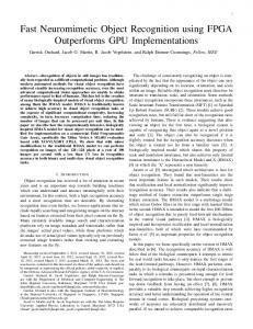
Experiments were performed on XM2VTS database. The XM2VTS database has been acquired at the University of Surrey. It contains four recordings of 295 subjects from the university. The volunteers visited the recording studio of the university four times at approximately one month intervals. On each visit (session) two recordings (shots) were made. The first shot consisted of speech whilst the second consisted of rotating head movements. Digital video equipment was used to capture the entire database [7]. Face tracking was applied on the head rotation shot videos that depict people that start from a frontal pose, turn their heads to their right profile, back to frontal pose then to the left profile. The images were then resized to 40 × 30. There are 1000 facial images captured this way. 500 of them are frontal and 500 non-frontal. Fig. 1 depicts some image

examples from the database. The first row contains frontal examples and the second row contains non-frontal examples.

Fig. 1. Image examples from database (1st row: Frontal, 2nd row: Non-frontal)

Due to the lack of another testing database we confined our analysis inside this database. Firstly, we conducted a 10-fold cross validation to compare PCA, LDA, CDA, PCA+LDA and PCA+CDA one against each other. Secondly, we conducted a series of reverse cross validation experiments, (by reducing the number of the training data samples), to assess the robustness of the algorithms and to find out whether they collapse. We actually reversed the training set with the test set, so that increasing the number of cross validation steps, the size of the training set decreased. 5.1

10-fold cross validation

On clustering step, we have used the Euclidean metric v ui=M uX 2 (xim − xin ) . d (xm , xn ) = t

(8)

i=1

and as similarity function the Gaussian similarity function which is defined as:   d (xm , xn ) . (9) fmn (σ) = exp − σ2 The parameter σ plays the role of the variance and determines the scale of the neighborhood of every data point. Our empirical study, has shown that σ = 0.25 · E (d (xm , xn )) is a value which offers intuitively satisfactory results. Using this value as σ, Spectral clustering systematically returned 2 clusters on non-frontal class and 3 clusters on frontal class at every step of cross validation procedure. In PCA+CDA, Spectral Clustering was performed after the PCA step, as proposed in [6]. The centroid image of every cluster is depicted on Fig. 2 (a). It is interesting to observe that the first cluster of non-frontal class consists of those faces that are turned to their left profiles and the second cluster consists of those turned to their right. Also, careful inspection shows that the 3 clusters of the frontal class consist of a group of dark faces, a group of medium brightness faces and a group of brighter faces respectively.

(a)

(b)

Fig. 2. (a) Centroid images of clusters. (First row: Non-frontal, Second row: Frontal), (b) 2D projection of the data

Using these 5 clusters extracted by the spectral clustering algorithm, CDA was capable of retaining up to 4 dimensions by keeping the four eigenvectors which correspond to the greatest four eigenvalues of C −1 R. Fig. 2 (b) depicts the projections of initial data points to the first two eigenvectors. The several clusters of the data are clearly shown on this figure. On table 1 we present the accuracy values that the several algorithms achieved at the 10-fold cross validation procedure. The approach that has been used is given on the 1st column. The proportion of the energy retained by PCA is given on the 2nd column. The accuracy value achieved by the specific method utilizing the NC and the NCC classifiers for PCA/LDA and CDA respectively, are given on the 3rd column. The accuracy values utilizing KNN classifier with K = 1 and K = 3, are given on the 4th and 5th column respectively. The bold value indicates the best performance. Its value is 98.9% and it has been reached by the PCA(95%)+CDA approach combined with the Nearest Cluster Centroid classifier. It is interesting to observe that PCA+KNN has similar performance to PCA+CDA approach and outperforms PCA+LDA approach. 5.2

Reducing the size of the training set

In the next experiment we compared the robustness of PCA(95%)+CDA+NC, PCA(95%)+LDA+NC and PCA+NC to the size of the training set. For the Spectral Clustering preprocessing we fixed the value of σ to 0.25 · E (d (xm , xn )) as before. Fig. 3 demonstrates how does the size of the training set affect the accuracy value of the several algorithms. On the horizontal axis the size of the

Table 1. 10-fold cross validation rates Dim. Reduction Classification approach P CA (%) NC/NCC 1-NN 3-NN P CA LDA

CDA

100 95 90 80 100 95 90 80

91.9 97.8 98.1 98.1 97.1 98 98.9 98.3 97.9

98.3 97.8 97.7 97.7 97 98.3 98.6 98.7 98.8

98.2 97.7 97.9 98.1 97.7 98 98.7 98.8 98.8

training set is given and on the vertical axis the accuracy value is depicted. There are three curves corresponding to the three aforementioned methods. Of course, as can be seen, as the size of the training set decreases, the performance of all three methods also decreases. However, it is clear that the PCA and LDA algorithms are more robust than CDA. The numbers on the edges of the PCA(95%)+CDA curve indicate the mean number of the clusters returned for the specific size of the training set. An explanation about the instability of the CDA algorithm can be given with the help of these numbers. We can see that while the size of the training set decreases, the number of clusters returned increases in a way that it no more represents the actual clustering structure of the data. For instance, there might arise a situation where a data point (e.g. outlier) constitutes a whole cluster on its own. In this case the CDA algorithm achieves the opposite results.

Fig. 3. Consecutive cross validation experiments

One reason for this unsuccessful clustering of the data is the fact that the Spectral Clustering algorithm is very sensitive to the choice of parameter σ. So, by fixing it to a standard value across the experiments makes the algorithm inflexible.

6

Conclusions

Frontal view recognition on still images has been explored in this paper. Subspace learning techniques (PCA, LDA and CDA) have been used for this purpose to achieve computationally easy and efficient results. Due to the low dimensionality of the reduced feature vectors, the use of complex classifiers like SVMs has been avoided and instead the K-Nearest Neighbor, Nearest Centroid and Nearest Cluster Centroid classifiers have been employed. Spectral Clustering performed on the XM2VTS database yielded interesting results which indicate that the problem of frontal view recognition is characterized by the existence of clusters inside the classes. 10-fold cross validation on the same database yielded an accuracy value equal to 98.9%, which was reached by the PCA(95%)+CDA approach. A set of eight consecutive experiments indicated that even though PCA+CDA beats PCA and PCA+LDA in 10-fold cross validation, however the latter two are more robust than CDA when the size of the training set decreases. Actually, what has been shown is the strong dependance of the CDA on the clustering of the data and the sensitivity of the clustering to the σ parameter.

References 1. Murphy-Chutorian, E., Trivedi, M.M.: Head pose estimation in computer vision: A survey. IEEE Transactions on Pattern Analysis and Machine Intelligence 31 (2009) 607–626 2. Azran, A., Ghahramani, Z.: Spectral methods for automatic multiscale data clustering. IEEE Conference on Computer Vision and Pattern Recognition (CVPR) 1(1) (January 2006) 190–197 3. von Luxburg, U.: A tutorial on spectral clustering. 17(4) (2007) 395–416 4. Jolliffe, I.: Principal Component Analysis. Springer Verlag (1986) 5. P. N. Belhumeur, J.P.H., Kriegman, D.J.: Eigenfaces vs fisherfaces: Recognition using class specific linear projection. IEEE Transactions on Pattern Analysis and Machine Intelligence 19(7) (1997) 711–720 6. wen Chen, X., Huang, T.: Facial expression recognition: a clustering-based approach. Pattern Recognition Letters 24 (2003) 1295–1302 7. Messer, K., Matas, J., Kittler, J., Luttin, J., Maitre, G.: XM2VTSDB: The extended M2VTS database. In: Second International Conference on Audio and Video-based Biometric Person Authentication (AVBPA). (1999) 72–77