Alfred P. Sloan Foundation; by a grant from the NSF under contract IRI-8719394; by. Hughes Aircraft Corporation (LJ90-074); by E.I. DuPont DeNemours and ...
MASSACHUSETTS INSTITUTE OF TECHNOLOGY ARTIFICIAL INTELLIGENCE LABORATORY A.I. Lab Memo 1259 (revised) C.B.I.P. Memo 59
October 1990
Model Based Recognition using Pruned Correspondence Search Thomas M. Breuel Abstract This paper presents a polynomial time algorithm (pruned correspondence search, PCS) for solving a wide class of geometric maximal matching problems, including the problem of recognizing 3D objects from a single 2D image. The PCS algorithm is connected with the geometry of the underlying recognition problem only through calls to a verification algorithm.
1
Introduction
This paper is concerned with an efficient algorithm for object recognition from visual data. We will study geometric recognition under under a bounded error model. This means determining, given sets of image and model points, whether there exists a transformation that will map each model point to within a given error bound of an image point. A more general version of this This research was sponsored by the ONR, Cognitive and Neural Sciences Division; by the Alfred P. Sloan Foundation; by a grant from the NSF under contract IRI-8719394; by Hughes Aircraft Corporation (LJ90-074); by E.I. DuPont DeNemours and Company; by the NATO Scientific Affairs Division (0403/87), and by ONR contract N00014–89–J–3139 under the DARPA ANN Technology Program. Support for the AI Laboratory’s research is sponsored by DARPA under Army contract DACA76–85–C–0010, and in part by ONR contract N00014–85–K–0124.
problem is to determine the size of the largest subsets of image and model points that can be brought into correspondence. In the case of visual object recognition, the “points” in the image and model are the location of features, such as line midpoints, vertices, singular points, centroids, etc. in the image and on the model. Bounded error models are interesting for several reasons (see [Norton, 1986], for a general discussion). In many applications, we are only concerned with the question of whether some value does not exceed certain tolerances, but the exact error is unimportant. Bounded error models also tend to be more robust and easier to apply than estimation techniques based on more specific models of error. [Baird, 1985], has analyzed the the problem of 2D visual object recognition under a bounded error model. He used linear programming to verify a set of correspondences between image and model points and found a maximal set of correspondence using a depth-first algorithm. Depth-first search algorithms to find maximal sets of correspondences have also been used by a number of other researchers (see, for example, [Ayache and Faugeras, 1986], [Grimson and Lozano-Perez, 1983]), often combined with heuristic methods for speeding up the search. While such algorithms have exponential worst case running times [Grimson, 1989], they are very popular because of their simple implementation and good performance in many practical situations. [Cass, 1990], has proposed an algorithm which is essentially a sweep of the arrangement (subdivision into cells, see [Edelsbrunner, 1987]) in transformation space generated by the constraints that arise from individual correspondences. [Alt et al., 1988], have proposed a similar algorithm. Such sweep based algorithms, while polynomial time in principle, have disappointing performance and cannot incorporate many of the known heuristics used for speeding up search based methods. This paper describes the pruned correspondence search (PCS) algorithm, an algorithm that combines the advantages of worst case polynomial time complexity with the good average case behavior of previous search-based algorithms.
2
B23 B17
m2
m1
B9
m3 T?
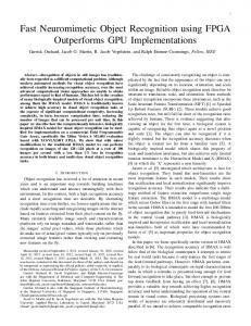
Figure 1: A formalization of the recognition problem with bounded error: Find the largest subset of points mi on the left such that there exists a transformation T (translation, rotation, scale) of the plane that maps the points into the error bounds Bj = bj + Ej given by image points bj together with error bounds given as sets Ej on the right.
2
The Geometry of Constraints
In this section, we review the geometrical view of transformations and bounded error matching that has originated with [Baird, 1985]. Assume that we are given a set of image points B = {b1 , . . . , bN } ⊆ R 2 and a set of model points M = {r1 , . . . , rM } ⊆ R 2 . A 2D transformation is given by a translation t and a rotation R. If we interpret the points as complex numbers, we can conveniently write the transformation of a model point into an image point as complex addition and multiplication: b(r) = t + Rr. Assume that error bounds on the location of image points are given as linear constraints. If the linear constraints are given by a vector u and a scalar 3
d, we then require for a transformation that is geometrically consistent with the pairing (correspondence) of a given image and model point that: u · (b − b(r)) ≤ d After a little manipulation, this can be rewritten as a linear constraint on the components of the transformation viewed as a vector in R 4 ([Baird, 1985]): ˜ u, r) ˜ b) · (t, R) ≤ d(d, C(u, If t is a 2-vector and R a matrix, then the constraints have the form: ˜ b) = [(uk )k=1,...,N , (ui bj )i=1,...,N ;j=1,...,M ] C(u, ˜ u, r) = d + u · r d(d, If t is a 2-vector and R is a rotation specified as a complex number, the constraints take the form: ˜ b) = [u0 , u1 , r · u, r × u] C(u, ˜ u, r) = d + u · r d(d, We see, therefore, that assuming a correspondence between a particular image point and a particular model point under a linear error constraint gives rise to a linear constraint on the set of allowable (“feasible”) transformations. The linear constraint on the transformation arising from a correspondence is geometrically a half-space in the four-dimensional space of transformations. If we impose several linear constraints on the location of an image point, the set of transformations compatible with a correspondence with that image point will form a convex polyhedron in transformation space, given by the intersection of the halfspaces corresponding to each individual linear constraint. Now consider the set of all possible correspondences between image and model points (there are at most M N of these). As we saw above, each correspondence will imply a convex polyhedron in transformation space. Correspondences that are compatible with one another, i.e., correspondences for which a transformation exists that allows all of them to be satisfied within 4
the given error bounds, will imply convex polyhedra that have a non-empty intersection. The problem of verification is that of determining, given a matching (a set of correspondences), whether there exists a transformation that aligns the matched points to within the given error bounds. In the transformation space view, this means that we have to determine whether the intersection of the constraint polyhedra implied by the individual correspondences is nonempty. A commonly used definition of the recognition problem (see, for example, [Baird, 1985], [Cass, 1990], [Grimson and Lozano-Perez, 1983]) is that of finding maximal subsets of the image and model points and correspondences between them that are consistent with some transformation.
3
The Algorithm
If some matching (set of correspondences) P is infeasible (geometrically inconsistent), no matching P 0 ⊇ P can be feasible. A natural approach to solving the recognition problem is therefore a depth first search; we start with an empty matching and add correspondences to it until the current matching becomes infeasible (i.e., until there is no transformation that is compatible with the current matching). We call a matching to which no other correspondence can be added without making it infeasible a leaf. Note that because matchings are sets, there is no particular order associated with the correspondences inside a leaf; different paths through the search tree may arrive at the same leaf. The set of all leaves forms a set of candidates for maximal matchings. Unfortunately, this simple algorithm has worst case exponential time complexity. The reason is that geometrically equivalent matchings may be reexplored by the search algorithm a large number of times. Consider the extreme example of matching n image points at the origin against n model points at the origin: in this case, there exist n! different (as sets) matchings, which would be explored by an unpruned depth first search algorithm; yet, there is only a single leaf. 5
The crucial idea presented in this paper is that regions in transformation space that have already been explored by the search algorithm can be represented concisely and efficiently as another set of correspondences, the adjoint set. When searching for a maximal matching using a depth-first algorithm, at each level in the search tree, we enlarge the current matching by adding another correspondence, test whether the resulting, larger, matching is geometrically feasible, and repeat this process recursively. In the PCS algorithm, in addition, we maintain the adjoint set, adding each correspondence to the adjoint set after it has been tried. And, instead of just testing whether a given matching is feasible, we also test whether we have not already explored all the geometric possibilities represented by that matching by testing whether there is some transformation that is inconsistent with every correspondence in the adjoint set but consistent with the current matching. In different words, by putting a correspondence between an image point with a model point in the adjoint set, we ensure that no transformations that map the model point to within the given error bounds of the image point will ever be reconsidered by the algorithm. In particular, this will guarantee that every leaf is considered only once by the algorithm. An algorithm based on these ideas is presented in Figure 2. In order to prove correctness and bound the running time of the PCS algorithm, we will prove that the function search adds each leaf to the set leaves exactly once. The function search has three arguments: the current matching (the current set of correspondences), the set remaining of correspondences that remain to be explored at the current level, and the set adjoint of correspondences that have already been explored at the current level in the search tree. We can think of the set current as representing a region Ic in transformation space that is given as the intersection of the correspondences contained in current, and of the set adjoint as representing a region Ua in transformation space formed by the union of the complements of the regions in transformation space implied by the correspondences in adjoint. The call to the function isfeasible with arguments current and adjoint tests whether the intersection of the regions Ic and Ua is non-empty. It is obvious that the function search can only add leaves to the set leaves. 6
It is also relatively straightforward to see that a leaf is always either fully contained in, or disjoint from, the regions Ic and Ua . Now, we will argue that search adds each leaf to the set leaves at most once. Because of the call to isfeasible at the beginning of search, only leaves that are contained in the region Ua can be added to the set leaves when search is called. If current is itself a leaf, it is trivially added only once. Otherwise, we have to consider the two recursive invocations of search. But the first recursive invocation adds the correspondence next to the set current, meaning that only leaves that are consistent with next can be found. The second recursive invocation adds next to the set of adjoints, meaning that only leaves that are inconsistent with next can be found. Therefore, the two recursive invocations of search must find disjoint sets of leaves. A similar inductive argument shows that search adds each leaf that is contained in Ic and not contained in Ua at least once to the set leaves. Because the initial call to search inside pcs is with an empty set current, representing all of transformation space, and an empty set adjoint, representing an empty region of transformation space that is excluded from further search, the function pcs actually returns a set of all leaves, with each leaf represented exactly once. Sometimes, a constraint that no image or model feature may be used twice in a matching is imposed. This can be expressed as a maximal bipartite graph matching problem between image and model features ([Cass, 1988]) which is solvable in low-order polynomial time ([Papadimitriou and Steiglitz, 1982]). Because of the way features are extracted from grey level images, imposing this constraint is rarely necessary in the 2D case.
4
2D and 3D Recognition
We have already discussed in detail the geometry of constraints and transformations in the case of matching 2D images against 2D models. With only little extra work, we can now say something about the average and worst case complexity of the PCS algorithm. [Megiddo, 1984], has demonstrated 7
function pcs(isfeasible,pairings) = let leaves = the empty set function isleaf(x) = test if x has no feasible successors function search(current,remaining,adjoint) = if not isfeasible(current,adjoint) then return else if isleaf(current) then append current to leaves else if remaining=the empty set then return else let next = first(remaining) in search({next}∪current, pairings−current, adjoint) search(current, rest(remaining), {next}∪adjoint) end in search(the empty set,pairings,the empty set) return leaves end
Figure 2: The pruned search algorithm. See the text for an explanation. that for any fixed dimension, the linear programming problem is solvable in linear time. Because of this, the verification problem in the case of recognition of 2D models from 2D images is actually solvable in linear time (i.e., O(N + M ), where N and M are the size of the image and model, respectively).
8
Node1
pruned
Node2
Node3
Node4
q2
q2
q3 q1
q1
...
q1
...
Figure 3: This figure illustrates schematically how the search tree for a maximal matching is pruned. The polygon indicates the region in transformation space that is compatible with the set of correspondences P1 at Node 1 and not excluded by the adjoint constraints A1 at the same node. The region of transformation space that a particular node is responsible for exploring is shown in dark grey. Node 2 is responsible for exploring the region where all constraints in P1 ∪ {q1 } are satisfied. Node 3 does not need to explore this region anymore; therefore, q1 has been added to the adjoint constraints when Node 3 is expanded. The search tree starting at Node 4 can be pruned in this example, because all the matchings containing q3 will already have been explored by nodes 2 and 3. For simplicity, let n = N M be the number of pairings between image and model points, and assume that there is a fixed maximum number of linear constraints associated with each model point. In practice, M , the number of model features, is often small and fixed, so that n varies linearly with the problem size. The function isfeasible that is called by the pcs algorithm actually has to be a little more powerful than a verification algorithm. It has to determine 9
whether the intersection Ic of one set of polyhedra with the union Ua of the complement of another set of polyhedra is non-empty. The running time of the isfeasible tests is polynomial, but dominates all the other work done inside each call to search. The number of leaves that can be returned by the pcs algorithm is at most1 as large as the number of cells that the arrangement of constraint polyhedra contains (see [Edelsbrunner, 1987], for a detailed discussion of linear arrangements). This can be shown by contradiction: if two different leaves were to fall into the same cell, then any correspondence from one could be added to the other, and one of them could not be a maximal matching. Since there are O(n) linear constraints and transformation space is 4 dimensional, the number of cells and the number of leaves are bounded by O(n4 ). This is a bound on the number of times that the function search will be called. For the recognition of rigid 3D objects from 2D images, the restrictions on the rotation R cannot be expressed in linear form anymore. The isfeasible algorithm now requires the simultaneous solution of linear inequalities together with a fixed set of quadratic equalities. One approach is to embed the manifold formed by all rotations and scaling matrices in a linear space, solve the verification problem in the larger space using linear programming, and then determine whether the intersection between the manifold and the polyhedron containing the feasible transformations is non-empty. Transformation space in the 3D case is five dimensional ( R 2 × R3 , where R 2 is the two dimensional Euclidean space of translations, and R3 is the three dimensional manifold of rotations). We expect the O(n) constraints to give rise to O(n5 ) leaves2 . Using homogeneous representations, similar results can be derived for perspective transformations. 1 This is a simple bound; in practice, the number of leaves is significantly smaller, and, in pathological cases, the number of leaves can be bounded by a polynomial in n even when the arrangement has a number of cells exponential in n. 2 The number of cells in the arrangement on the surface of the manifold of rotations may be larger.
10
Figure 4: A typical recognition problem. The edges of the images were extracted from a grey level image using an implementation of the Canny edge detector and approximated by straight line segments using a splitting algorithm. Shown is a cluttered scene with 12 widgets. The best match for one of the widgets (in terms of model boundary length accounted for in the image) is shown in light grey. Arbitrary translations, rotations, scaling, and occlusions were allowed. Model and image features were required to match within an error of 5 pixels. Other algorithms, such as heuristic search termination or incompletely pruned algorithms, either did not find the optimal solution, or could not be run to completion because of the combinatorial explosion of the number of possible matchings.
5
Discussion
Previous correspondence search-based recognition algorithms had worst case, and sometimes even average case, exponential time behavior in the presence of clutter and occlusion ([Grimson, 1989]). The PCS algorithm described in this paper has worst case polynomial time complexity in all cases.
11
The only other known recognition algorithms under the bounded error model with polynomial time complexity are sweeps of the arrangement of constraints on transformations. The PCS algorithm appears to be more efficient for the average case compared to such methods. It also explores the set of leaves in a more natural and useful order; likely candidates for solutions can be moved early into the search tree. A variety of standard techniques, such as configuration based matching or testing for consistency among small numbers of features and caching the result, used for speeding up correspondence searchbased recognition algorithms, can be incorporated into the PCS algorithm.
References [Alt et al., 1988] Alt H., Mehlhorn K., Wagener H., Welzl E., 1988, Congruence, Similarity, and Symmetries of Geometric Objects., Discrete and Computational Geometry. [Ayache and Faugeras, 1986] Ayache N., Faugeras O. D., 1986, HYPER: A New Approach for the Recognition and Positioning of Two-Dimensional Objecs, IEEE Transactions on Pattern Analysis and Machine Intelligence, PAMI-8(1):44–54. [Baird, 1985] Baird H. S., 1985, Model-Based Image Matching Using Location, MIT Press, Cambridge, MA. [Cass, 1988] Cass T. A., 1988, Robust Parallel Computation of 2D ModelBased Recognition, In Proceedings Image Understanding Workshop, Boston, MA, Morgan and Kaufman, San Mateo, CA. [Cass, 1990] Cass T. A., 1990, Feature Matching for Object Localization in the Presence of Uncertainty, A.I. Memo No. 1133, Artificial Intelligence Laboratory, Massachusetts Institute of Technology. [Edelsbrunner, 1987] Edelsbrunner H., 1987, Algorithms in Combinatorial Geometry, Springer Verlag. [Grimson and Lozano-Perez, 1983] Grimson W. E. L., Lozano-Perez T., 1983, Model-Based Recognition and Localization From Sparse Range or Tactile Data, Technical Report A.I. Memo 738, MIT. [Grimson, 1989] Grimson W. E. L., 1989, The Combinatorics of Heuristic Search Termination for Object Recognition in Cluttered Environments., 12
A.I. Memo No. 1111, Artificial Intelligence Laboratory, Massachusetts Institute of Technology. [Megiddo, 1984] Megiddo N., 1984, Linear Programming in Linear Time when the Dimension is Fixed, J. Assoc. Comput. Mach. (USA), 31(1). [Norton, 1986] Norton J. P., 1986, An Introduction to Identification, Wiley. [Papadimitriou and Steiglitz, 1982] Papadimitriou C. H., Steiglitz K., 1982, Combinatorial Optimization, Prentice Hall.
13