1 â (n â 1)Ç«, if i = j ; Ç«, if i = j . It represents a special case of the house of cards model of mutation [19,20] fre- quently used in theoretical population genetics.
Full Characterization of a Strange Attractor Chaotic Dynamics in Low-dimensional Replicator Systems
By Wolfgang Schnabl, Peter F.Stadler, Christian Forst and Peter Schuster ∗
Institut f¨ ur theoretische Chemie der Universit¨at Wien
Mailing Address: Prof.Peter Schuster, Institut f¨ ur theoretische Chemie der Universit¨at Wien W¨ahringerstraße 17, A 1090 Wien, Austria Phone: (0222) 43 61 41 / 78 D Bitnet: A8441DAM@AWIUNI11
W.Schnabl et al.: Chaotic Attractor
Page 1
Abstract Two chaotic attractors observed in Lotka-Volterra equations of dimension n = 3 are shown to represent two different cross-sections of one and the same chaotic regime. The strange attractor is studied in the equivalent four dimensional catalytic replicator network. Analytical expression are derived for the Ljapunov exponents of the flow. In the centre of the chaotic regime the strange attractor is characterized by numerically computated R´enyi fractal dimensions, Dq (q = 0, 1, 2) = 2.04, 1.89 and 1.65 ± 0.05 as well as the Ljapunov dimension DL = 2.06 ± 0.02. Accordingly it represents a multifractal. The fractal set is characterized by the singularity spectrum. Two routes in parameter space leading into the chaotic regime were studied in detail, one corresponding to the Feigenbaum cascade of bifurcations. The second route is substantial different from this well known pathway and has some features in common with the intermittency route. A series of one-dimensional maps is derived from a properly chosen Poincar´e cross-section which illustrates structural changes in the attractor. Mutations are included in the catalytic replicator network and the changes in the dynamics observed are compared with the predictions of an approach based on pertubation theory. The most striking result is the gradual disappearance of complex dynamics with increasing mutation rates.
W.Schnabl et al.: Chaotic Attractor
Page 2
1. Introduction
The search for chaotic dynamics became an issue in many scientific disciplines from physics to biology. The relevance of strange attractors in modeling real systems and the problem how to trace chaos in the experimental data were important questions already five years ago [1] and remained in the centre of interest since then [2-4] . Numerical evidence for strange attractors was found in many model equations but unlike simple attractors they cannot be characterized by a few coordinates or coordinates and frequencies. In the poineering works of several groups efficient techniques to analyse chaotic dynamics and fractal sets were developed (For a recent review of the available repertoire of methods see [5,6]).
In order
to provide a sufficiently detailed basis for the comparison of model calculations and experimental data full characterization of strange attractors is required. We present such a study on a chaotic attractor which appears in the solutions of a differential equation which is of interest in biophysics and in theoretical ecology as well as in other disciplines. Autocatalytic reaction networks which involve two classes of catalytic processes – autocatalytic instruction for reproduction as well as material and process specific catalysis – were postulated as models for studies on prebiotic and early biological evolution scenarios [7,8]. Now they serve also as simple models showing the characteristic features of nonlinear dynamics in very different fields like molecular biology, population genetics, theoretical ecology or dynamical game theory [9] . Qualitative analysis and systematic numerical investigations revealed a very rich dynamics of the corresponding kinetic differential equations [10] . The name
W.Schnabl et al.: Chaotic Attractor
Page 3
replicator equations was coined for these systems because they reveal several unique and – in the standardized form to be discussed in the next section 2 – fairly easy to proof features [11] . The four species replicator system shows chaotic dynamics for certain parameter values [12] . According to Hofbauer [13] this autocatalytic network with four species is – apart from a transformation of the time scale – equivalent to a three-species Lotka-Volterra equation. Possible existence of very complex dynamical behaviour in Lotka-Volterra models was predicted by Smale [14] . Indeed two different strange attractors were reported for the LotkaVolterra system [15-18],
which describes communities of one predator species
living on two prey species. In this contribution we shall show that the two strange attractors lie on different cross-sections through one and the same chaotic regime. The number of degrees of freedom is minimal for the occurrence of strange attractors and hence the chaotic regime in question houses the simplest strange attractors possible in Lotka-Volterra and replicator equations – replicator systems have normalized variables and hence the number of independent degrees of freedom is the number of species but one.
2. The replicator model
Replicator equations are based on the simplest possible molecular mechanism of catalysed replication and mutation. The basic reactions are of the form Qkj ·Aji
(A) + Ij + Ii
−−−→
Ij + Ik + Ii
;
i, j, k = 1, . . . , n .
(1)
W.Schnabl et al.: Chaotic Attractor
Page 4
Herein Ij is the template which is replicated and Ii the catalyst, (A) represents an overall notation for substrates needed for replication. It is assumed that the substrates are present in excess – their concentration are buffered and hence do not change during the course of reactions. There are n3 possible reactions producing the n different species Ik (k = 1, . . . , n) of the autocatalytic reaction network. Clearly it is very hard – if not impossible – to handle such a large number of parameters. In order to be able to analyse the reaction network simplifying assumptions are inevitable. It is straight forward to treat catalysed replication and mutation as independent superpositions: mutation frequencies depend on template (Ij ) and target (Ik ), but not on the catalyst (Ii ). The remaining 2n2 rate parameters are properly understood then as elements of two n × n matrices: a replication rate . . matrix A = (Aji ) and a mutation matrix Q = (Qkj ). The rate constants of the individual reactions are products of a replication and a mutation factor. Qkj · Aji , expressing the following sequence of processes: Ii catalyzes the replication of Ij which yields Ik as an error copy. Error-free replication of species Ij – described by equ.(1) with Ik ≡ Ij – is assumed to occur with frequency Qjj . A mutation from Ij to Ik , (k 6= j) occurs with frequency Qkj . Every copy has to be either correct or a mutant and thus Q is a stochastic matrix (
Pn
k=1
Qkj = 1 ∀ j = 1, . . . , n).
Concentrations of individual species are denoted by ck = [Ik ]. As variables we .P n use relative – or normalized – concentrations: xk = ck j=1 cj which obviously fulfil
Pn
k=1
xk = 1.
W.Schnabl et al.: Chaotic Attractor
Page 5
Mass action kinetics applied to the autocatalytic reaction-mutation network (1) yields an ODE of the form n X dxk = x˙ k = Qki Aij xi xj − xk Φ, dt i,j=1
k = 1, . . . n
(2)
where an automatically adjusted dilution flux
Φ=
n X
Aij xi xj
i,j=1
is introduced in order to keep the sum of relative concentrations normalized to unity. The physically meaningful domain of equ.(2) is the simplex . Sn =
If Aij ≥ 0,
�
(x1 , . . . , xn ) | xi ≥ 0,
n X
xi = 1
i=1
�
i, j = 1, . . . n then Sn is a compact, foreward invariant set for the
ODE (2). An intensity of mutation can be measured by the mean mutation rate ǫ: . ǫ=
n X 1 Qij n(n − 1)
(3)
i6=j i,j=1
Throughout this paper we use a particularly simple type of the mutation matrix
Qij =
�
1 − (n − 1)ǫ, if i = j ; ǫ,
if i 6= j .
It represents a special case of the house of cards model of mutation [19,20] frequently used in theoretical population genetics.
W.Schnabl et al.: Chaotic Attractor
Page 6
The important special case of error-free replication is represented by a unit mutation matrix, Q = id. Then equ.(1) is turned into the well known replicator equation: x˙ k = xk
�X n
Aki xi −
n X
Aij xi xj
i,j=1
i=1
�
(4)
The linear replicator equation (4) for n is flow-equivalent to the n − 1 species Lotka-Volterra equation: � � n−1 X βkj yj ; y˙ k = yk αk +
k = 1, . . . , n − 1 .
(5)
i=1
The variables are related by means of the transformation introduced by Hofbauer [13]: yk =
xk xn
for
k = 1, . . . , n − 1 .
(6)
3. The chaotic regime in parameter space
Two distinct chaotic attractors were found in Lotka-Volterra equations for three species: Vance [17] discovered a “quasi-cyclic” trajectory in a one predator two prey model and Arneodo, Coullet and Tresser [15] found a one parameter family of strange attractors (ACT-attractor). We used Hofbauer’s transform to construct the replicator equations which are equivalent to the models mentioned above. Then a barycentric transform [21] was applied to Vance’s model in order to shift the interior fixed point into the centre of the simplex S4 – the point c = 41 (1, 1, 1, 1).
W.Schnabl et al.: Chaotic Attractor
Page 7
A barycentric transformation can always be found if the replicator equation
z˙k = zk
�X n
bki zi −
i=1
n X
bij zi zj
i,j=1
�
ˆ = (ˆ has an interior fixed point z z1 , zˆ2 , . . . , zˆn ). It can be shown [22] that there exists a diffeomorphism which relates this replicator equation to another one in the notation of equ.(4) with bij zˆj
Aij =
and
ˆ = x
� 1 1, 1, . . . , 1 . n
Both the ACT family and the Vance attractor (V) correspond to nonrobust phase-portraits because of zero or almost zero (see e.g. A24 or A43 in AV ) offdiagonal elements in the reaction matrices A. In order to make the numerical computations easy to reproduce all parameter values were rounded to three digits. Then the Vance model has a replication matrix 0 0.063 0 0.437 0 −0.036 −0.001 0.537 AV = −0.535 0.38 0 0.655 0.536 −0.032 −0.004 0
(7)
and the ACT attractors are found at
AACT
0 1.1 = −0.5 1.7 + µ
0.5 0 1 −1 − µ
−0.1 0.1 −0.6 0 0 0 −0.2 0
(8)
Note that we use a parameter µ which corresponds to µ − 1.5 in [15]. In order to find out whether or not these two attractors are related in the twelve-dimensional parameter space we performed a systematic numerical survey
W.Schnabl et al.: Chaotic Attractor
Page 8
in the two-dimensional subspace (µ, ν ) which connects the two models: A(µ, ν) =
0 1.1 − 0.563ν = −0.5 − 0.035ν 1.7 + µ − 1.164ν
0.5 − 0.437ν 0 1 − 0.62ν −1 − µ + 0.968ν
−0.1 + 0.1ν −0.6 + 0.564ν 0 −0.2 + 0.196ν
0.1 + 0.337ν −0.001ν 0.655ν 0
We note that all three matrices of replication constants fulfil
P4
j=1
(9)
Aij = 0.5 –
a property which will be used together with the existence of a fixed point in the centre of the simplex later on. In the (µ, ν)-plane the ACT model lies on the line −0.2 ≤ µ ≤ 0.05 and ν = 0. The Vance-attractor is close to the point (0, 1). Both models are embedded in a Σ-shaped two-dimensional manifold of strange attractors (fig.1). In scanning through the manifold we could not find any sudden changes in the shape of the attractor. The mean revolution time also varies in apparently continuous manner all over the chaotic regime.
Fig. 1: A two-dimensional cross-section through the chaotic regime of equ.(4). The cross-section is defined by the two parameters µ and ν in the replication matrix A (9).
A common feature of all phase portraits exhibiting chaotic behaviour (attractive or only transient) is a saddle focus P123 on the [1, 2, 3]-plane, which represents the stable manifold. The unstable manifold thus points into the interior of the ˇ simplex. We found that Silnikov’s condition [23] is always satisfied: the real positive eigenvalue is larger in magnitude than the real parts of the two complex
W.Schnabl et al.: Chaotic Attractor
Page 9
conjugate eigenvalues. Although there is no homoclinic orbit possible for P123 , a ˇ close relation to Silnikov’s condition is evident, as was pointed out by Arneodo et al. [16]: there is a heteroclinic orbit involving three saddles instead of one and this orbit replaces the homoclinic one. For generalized Lotka-Volterra models with additional cubic terms Samardzija and Greller [24] found a different type of chaos arising from a fractal torus. For small values of µ the fixed point in the centre of S4 (c) is stable. Chaos is reached via a Hopf bifurcation and a subsequent cascade of period doubling bifurcations. At first the limit cycle, and then the chaotic attractor, both grow steadily with increasing µ-values. At a parameter value around µ = 0.21 the chaotic attractor collides with the stable manifold of a saddle on the [1, 2, 4]-plane and disappears suddenly. This behaviour is known as limit crisis [25] : at the bifurcation point we find a heteroclinic orbit connecting the [1, 4]-saddle, a saddle on the [1, 2]-edge, and the saddle-focus in the [1, 2, 3]-plane (fig.2). The evidence for the orbit is derived from numerical integration. We cannot provide an analytical proof for the saddle connection between the saddle focus and P12 . The saddle connections on the boundary follow from the invariance of the subsimplices and the classification of the flow of three component replicator equations [26,27]. Beyond the limit crisis we find a field of transient chaos: the trajectory seems to draw an image of the chaotic attractor which in parameter space lies on the other side of the limit crisis before it ends up in a stable fixed point. For small values of ν the frequency of the oscillations increases with decreasing parameter values – revolution times become shorter and shorter. Eventually the
W.Schnabl et al.: Chaotic Attractor
Page 10
attractor collides with the stable manifold of the saddle on the [1, 2]-edge. The invariant hyperplane
P4
k=1
xk = 1 is a repellor in this area and therefore integration
is extremely sensitive to numerical errors.
Fig. 2: A sketch of fourteen flows on the boundaries of the simplex S4 which can coexist with the chaotic attractor in the interior. The numbers (1) to (14) are used as markers in fig.1 to indicate where the phase portraits occur in parameter space.
The chaotic attractor in the interior of the simplex S4 coexists with a rather large variety of robust flows on the surface. Fig.2 shows fourteen boundary-flows consistent with chaos on the (µ, ν)-plane. Fig.3 sketches the phase portraits of the ACT and the Vance model together with a typical chaotic trajectory for each system.
Fig. 3: Phase portraits and chaotic trajectories in the Vance (7) and the ACT model (8).
Direct evidence from the inspection of computed trajectories was supplemented by Fourier transformation [28] . Some typical examples of Fourier spectra in periodic and chaotic regimes of our attractor are shown in fig.4. They are used as a sensitive indicator of the occurence of chaos. In the four spectra chosen we observe a complete transition from a periodic window into the chaotic regime caused by a small change in the parameters (∆µ < 0.02).
W.Schnabl et al.: Chaotic Attractor
Page 11
Fig. 4: Fourier spectra of selected trajectories of the replicator model (9) with the parameter values ν = 0 and µ = −0.0536 (A), -0.0529 (B), -0.05 (C) and -0.04 (D).
4. Measures of the chaotic attractors
The most common measure for a chaotic attractor is the spectrum of Ljapunov � �� exponents [29] . Let J(t) = ∂F x x(0), t be the Jacobian of the vectorfield F
along a trajectory with starting point x(0). Now we define an operator Z t o n . ˆ J(τ )dτ . L(t) = T exp
(10)
0
ˆ has to be introduced since Jacobian matrices evalThe time ordering operator T uated at different times – J(τ ) and J(τ ′ ) – usually do not commute. Let µi (t) be the eigenvalues of L(t), then the Ljapunov exponents are given by ln kµi (t)k . t→∞ t
λi = lim
(11)
In most cases it is not possible to calculate Ljapunov exponents for the flows of differential equations analytically. An appropriate numerical algorithm has been given by Bennetin et al. [30] , a well tested fortran program is available in the literature [31] . In the four-species replicator system there are three physical dimensions imbedded in a four-dimensional state space. The hyperplane Σ4 =
n
4 X o xi = 1 x ∈ IR 4
i=1
W.Schnabl et al.: Chaotic Attractor
Page 12
is invariant. Accordingly L(t) has three eigenvectors ξ~i lying in this plane and their P (i) components fulfil k ξk = 0. The fourth eigenvector is pointing out of the hyperplane. Thus we expect to find three physical meaningful Ljapunov exponents.
If all three of them are negative the attractor is a sink. For a periodic, quasiperiodic or chaotic attractor at least one eigenvalue has to be zero: this exponent corresponds to an eigenvector which points in the direction of the trajectory. In particular, we have for periodic orbits λ1 ≤ λ2 < 0, λ3 = 0, for quasiperiodic orbits λ1 < 0, λ2 = λ3 = 0 and finally for a chaotic attractor one Ljapunov exponent is negativ, one is zero and one is positiv, λ1 < 0, λ2 = 0, λ3 > 0. The sum of all Ljapunov exponents fulfils the equation Z n X � 1 t div F x(τ ) dτ λi = lim t→∞ t 0 i=1
(12)
For error-free replication – if the mutation matrix Q = id – the divergence div F reduces to div F =
n X
Akj xj − (n + 2)
n X
Aij xi xj .
(13)
i,j=1
k,j=1
¯ is defined by The mean flux Φ ¯ = lim 1 Φ t→∞ t
Z
t
n X
Aij xi (τ )xj (τ )dτ
0 i,j=1
If the replicator equation is permanent [11,32,33] – or at least if the trajectory converges to an interior fixed point – we have Z 1 t x˙ k 1 n log xk (t) − log xk (0) o 0 = lim = dτ = lim t→∞ t 0 xk t→∞ t t Z Z n n X 1 t X 1 t xj (τ )dτ − lim Aij xi (τ )xj (τ )dτ = = Akj lim t→∞ t 0 t→∞ t 0 i,j=1 j=1 =
n X j=1
¯ Akj x ¯j − Φ
W.Schnabl et al.: Chaotic Attractor
Page 13
Since the last line is the equation fulfilled by the coordinates of the interior fixed point we have 1 x ¯j = lim t→∞ t
Z
t
xj (τ )dτ = x ˆj
(14)
0
where x ˆ = (ˆ x1 , x ˆ2 , · · · , x ˆn ) is the interior fixed point if it exists. Its coordinates fulfil the equations n X
¯ , Aij x ˆj = Φ
j
and hence we have n X
¯ Aij x ˆj = n · Φ
∀ i = 1, . . . , n .
i,j=1
Accordingly we find 1 lim t→∞ t
Z
t
0
� � ¯ . div F x(τ ) dτ = −2 · Φ
(15)
Finally we are left with the following relation derived from equ.(12) for the sum n 2 X Aij . λi = − 2 n i,j=1 i=1
n X
(12a)
1 holds Since we applied the barycentric transformation to our model, x ˆj = n for all coordinates and we obtain ¯ = Φ
n 1 X Aij . n2 i,j=1
Using the numerical values of (9) the sum of the four Ljapunov exponents becomes P4
i=1
λi = − 41 . The eigenvector pointing in the direction (1, 1, 1, 1) is denoted by 1 1 1 e = 2 1 1
W.Schnabl et al.: Chaotic Attractor
Page 14
The corresponding Ljapunov exponent (λ4 ) can be calculated analytically. Let us consider the orbit of the linearized model starting from x(0) = e which to first order in time is given by x(τ ) = e + τ · ∂F · e + O(τ 2 ) .
Then we obtain for the Ljapunov exponent N � 1 X log{τ · < e|I + ∂F x(jτ ) |e >} = N→∞ τ →0 N τ j=1
λ4 = lim lim
N � 1 X = lim lim τ · < e|∂F x(jτ ) |e > = N→∞ τ →0 N τ j=1 Z t � 1 ¯ = lim < e|∂F x(τ ) |e > dτ = −Φ t→∞ t 0
The last equation is derived straightway by explicit evaluation of the integrand as the sum over all elements of the Jacobian. One obtains the same result −Φ(τ ) for ¯ every time τ and hence λ4 = −Φ. Thus we have in case of our model: 4 X
λi = −
i=1
1 4
and
λ4 = −
1 . 8
(16)
In the chaotic regime it is sufficient therefore to compute the largest Ljapunov exponent λ1 . All other exponents are obtained from: 1 λ2 = 0 , λ3 = − − λ1 8
and λ4 = −
1 . 8
(17)
In fig.5 we show the largest Ljapunov exponent (λ1 ) of the strange attractor as a function of the parameter µ.
W.Schnabl et al.: Chaotic Attractor
Page 15
Fig. 5: The largest Ljapunov exponent λ1 of the vector flow defined by equ.(9). In order to show a representative cross-section through the chaotic regime we chose ν = 0.
From the Ljapunov exponents we can calculate an estimate for the fractal dimension of our attractor:
DL
� � λ1 = 2 1 + 12λ1 2 − λ3 1 + 8λ1 = 1 0
if λ1 > 0 , if λ1 = 0 and if λ1 < 0 .
(18)
From fig.5 we obtain λ1 = 8 × 10⁻³ for the highly developed chaos at µ = ν = 0 and compute a dimension of DL = 2.06 with an estimated numerical uncertainty of ±0.02 at this point. In order to study the fractal nature of the attractor quantitatively we computed also generalized or R´enyi dimensions, Dq , which correspond to the scaling exponents of the q-th moments of the attractor’s measure [34,35]. The attractor is covered by M (ℓ) cells with edges of length ℓ. By pi we denote the probability to find a point of the attractor in cell number i (i = 1, . . . , M (ℓ)). Then R´enyi dimensions are obtained from
Dq
PM (ℓ) log i=1 piq log C q (ℓ) = lim = lim , ℓ→0 (q − 1) log ℓ ℓ→0 (q − 1) log ℓ
(19)
. PM (ℓ) where we introduced the definition C q (ℓ) = i=1 piq . In order to circumvent an indeterminate expression in the denominator the R´enyi dimension D1 is obtained by taking the limit limq→1 Dq = D1 . For the actual calculations we can rewrite
W.Schnabl et al.: Chaotic Attractor
Page 16
the sum over the pi ’s in terms of the probability p˜i of the trajectory to cross a box of size ℓ around the iterate x(tj ). We make use of the equation M (ℓ)
lim
ℓ→0
X
piq =
i=1
N 1 X q−1 p˜j N→∞ N j=1
(20)
lim
and find that the latter probability is given by N 1 X Θ(ℓ − kxi − xj k) , N→∞ N i=1
p˜j = lim
(21)
where Θ is used for the Heaviside function: Θ(x − x0 ) =
�
0 1
for x < x0 , for x ≥ x0 .
Thus we are left with the easier to compute expression �q−1 M (ℓ)� M (ℓ) 1 X X Θ(ℓ − kxi − xj k) . C (ℓ) = lim N→∞ N q i=1 j=1 q
(22)
In the limit q → 1 we find for the R´enyi dimension � X � N N X 1 1 D1 = lim lim log Θ(ℓ − kxi − xj k) . N→∞ ℓ→0 N · log ℓ N j=1
(23)
i=1
For the lowest integer q values the R´enyi dimensions Dq are equal to Hausdorff dimensions (q = 0), information dimensions (q = 1) and correlation dimensions (q = 2). The evaluation of R´enyi dimensions turned out to be extremely time consuming and therefore we restricted computations to one point right in the centre of the chaotic regime (µ = ν = 0). In order to calculate the numbers C q (ℓ) the trajectory was decomposed into a time series X =
�
Xi = x(ti ) ∀ i = 1, 2, . . . , N
(24)
W.Schnabl et al.: Chaotic Attractor
Page 17
with t1 < t2 < . . . < tN . Some ten thousand points are required which have to be distributed independently along a trajectory. This condition can be met by collecting subsequent points which are separated by at least one full revolution on the attractor. We record mean revolutions times of the order tR ≈ 102 for our attractor and hence the trajectory had to be followed up to t ≈ 2 × 10⁵ . Inserting the fractal set obtained into equs.(22) and (23) we found D0 = 2.04 ,
D1 = 1.89 and
D2 = 1.65 .
The estimated numerical uncertainty of our values amounts to ±0.05. We note that the Hausdorff dimension of the attractor is the same as the Ljapunov dimension within the error limits and fulfils the condition DL ≥ D0 . Fractal sets can be characterized by the scaling properties of normalized distributions or measures lying upon them [36] . We briefly repeat the basic expressions and relations. Scaling properties are expressed in terms of singularity strengths α and a function f (α) which reflects the density of their distribution. The spectrum of singularities is given by the possible range of α values and the density f (α). In order to define these quantities we cover the attractor with boxes of size ℓ and denote the number of points inside the ith box by Ni . Then the probability that this box contains a point of the attractor’s time series (24) is given by � � Pi (ℓ) = limN→∞ Ni N . The local singularity strength αi is now given as the scaling exponent Pi (ℓ) ∝ ℓαi . The singularity strength αi thus varies with the re-
gion of the attractor on which it is taken. Its probability density - the probability to encounter a value of α between α ˜ and α ˜ + dα ˜ – is given by � ˜ Prob α ˜