12
P. POMĚNKA, Z. RAIDA, METHODOLOGY OF NEURAL DESIGN: APPLICATIONS IN MICROWAVE ENGINEERING
Methodology of Neural Design: Applications in Microwave Engineering Petr POMĚNKA, Zbyněk RAIDA Dept. of Radio Electronics, Brno University of Technology, Purkyňova 118, 612 00 Brno, Czech Republic
[email protected] Abstract. In the paper, an original methodology for the automatic creation of neural models of microwave structures is proposed and verified. Following the methodology, neural models of the prescribed accuracy are built within the minimum CPU time. Validity of the proposed methodology is verified by developing neural models of selected microwave structures. Functionality of neural models is verified in a design – a neural model is joined with a genetic algorithm to find a global minimum of a formulated objective function. The objective function is minimized using different versions of genetic algorithms, and their mutual combinations. The verified methodology of the automated creation of accurate neural models of microwave structures, and their association with global optimization routines are the most important original features of the paper.
Keywords Artificial neural networks, genetic algorithms, methodology of developing neural models Bayesian regularization, Levenberg-Marquardt algorithm.
1. Introduction In the microwave frequency band, dimensions of components are comparable to the wavelength. Therefore, Maxwell equations have to be solved when analyzing microwave structures (so called full-wave analysis) [1], [2]. CPU-time demands of the full wave analysis are its basic problem. In order to reduce CPU-time requirements, artificial neural networks can be used: the neural network is trained to provide the same results like the full-wave analysis, and therefore, the numerical model can be replaced by the neural one [3]–[6]. CPU-time modest neural models can be combined with genetic algorithms to perform the global optimization of the designed structure [3]–[6]. While genetic algorithms are well-described in the open literature, e.g. [7]–[9], the methodology of creating neural models has not been published yet.
In section 2 of this paper, the proposed methodology of creating neural models is described, and its application is illustrated by developing the neural model of a frequency selective surface (FSS). In section 3, the neural model of FSS is associated with genetic algorithms to obtain a tool for the global design. The section 4 concludes the paper.
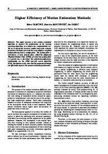
2. Neural Design Neural networks have been widely used in electronics since middle eighties. Their development has been related to the rapid grow of a potential computational power of computers. In the area of microwave applications, neural networks have been used for computing resonance frequency of microstrip antennas [10], modeling microwave circuits [11], [12], computing effective permitivity of microwave lines [13], and many other applications. Nevertheless, the general methodology of their utilization has been missing. We have developed methodologies for creating neural models of scatterers (represented by FSS), transmission lines (represented by a microstrip in layered media), and planar antennas (represented by a microstrip dipole). Common features of those methodologies have been extracted into a general recipe [14]. The basic principles of the developed methodology are demonstrated on modeling a FSS, which consists of a periodic array of perfectly electrically conductive rectangular patches on an infinite substrate. Parameters of the substrate are identical with the parameters of the surroundings. b y0 a
A B Fig. 1. Frequency selective surface.
RADIOENGINEERING, VOL. 15, NO. 2, JUNE 2006
13
The described FSS is analyzed by the spectral domain method of moments to build a training set. Input patterns are created by doublets [b, B] where b is the width of the rectangular patch and B is the width of the substrate cell containing the patch (Fig. 1). Output targets are formed by triplets [f1, f2, f3] where f2 is the frequency of the first maximum of the module of reflection coefficient, and f1 and f3 are frequencies of 3 dB decrease of the module of reflection coefficient. In analysis, we assume the Floquet mode (0, 0), and the vertical polarization of the incoming wave. The neural model is going to be built over the input space b ∈ and B ∈ . Initially, the input space is roughly sampled using the equidistant sampling (the step length was set to 3 mm in our case). Hence, the initial input pattern has consisted of 3 × 5 values. In the following steps, the sampling is refined in regions exhibiting an unacceptably high modeling error.
77
5
5
63
Max. number of cycles
4
-6
501
500
-6
501
500
-5
501
500
-6
501
500
-1
132
500
-1
124
500
-1
136
500
-6
501
500
-6
501
500
-6
501
500
-6
501
500
-6
529
600
-6
474
600
-1
130
600
-1
130
600
Accuracy achieved
Efficiently used parameters [%]
4
Cycles performed
2
Neurons in nd the 2 layer
1
Neurons in st the 1 layer
Realization No.
The initial architecture of the feed-forward neural network has contained 2 hidden layers each having 4 neurons. The network has been trained to provide the same results like the full-wave analysis: the maximum number of cycles has been set to 500, the desired accuracy to 10-6, and Bayesian regularization has been used for training (see Tab. 1.). Finishing the training, the model accuracy has been tested by comparing network outputs and analysis results for the sampling step 0.5 mm (thus, the input space is represented by the matrix consisting of 13 × 25 values). If an unacceptably high modeling error is exhibited, the neural network architecture is refined.
6.77 ⋅ 10 4.29 ⋅ 10 1.24 ⋅ 10
3
5
5
57
4
5
5
62
3.99 ⋅ 10
5
5
6
04
5.62 ⋅ 10
6
5
6
04
7
5
6
04
8
6
6
48
5.62 ⋅ 10 5.62 ⋅ 10 4.72 ⋅ 10
9
6
6
49
3.43 ⋅ 10
10
6
7
48
4.45 ⋅ 10
11
5
6
43
2.91 ⋅ 10
12
5
6
52
3.53 ⋅ 10
13
5
6
56
3.05 ⋅ 10
14 15
5 5
6 6
04 04
5.62 ⋅ 10 5.62 ⋅ 10
Tab. 1. Results of searching the optimal neural network architecture using Bayesian regularization.
Let us assume that the optimal architecture of the neural model has been found. This fact does not necessarily mean that the neural model provides results with the training accuracy (column Accuracy Achieved in Tab. 1). For input patterns, which differ from the training ones, the modeling error might be much higher. The optimal architecture therefore means that the modeling accuracy is sufficient (below 5 %), and that the number of efficiently used parameters of the neural network is within 50 % to 80 %. For the optimal architecture of the neural model, further tests and improvements have been performed: • The same architecture has been trained using Levenberg-Marquardt algorithm to refine network settings; • The input set has been enriched by additional training points in regions, where the desired accuracy has not been reached (training has been repeated by both the Bayesian regularization and the Levenberg-Marquardt algorithm); • A small number of neurons (one or two) has been removed from the first hidden layer or the second one to prevent over-training [16]–[18], and consequently, the network has been trained with Levenberg-Marquardt algorithm;
Fig. 2. An error of the FSS neural model trained by Bayesian regularization, Δb = ΔB = 3 mm.
Fig. 3. An error of the FSS neural model trained by LevenbergMarquardt algorithm, Δb = ΔB = 3 mm.
14
P. POMĚNKA, Z. RAIDA, METHODOLOGY OF NEURAL DESIGN: APPLICATIONS IN MICROWAVE ENGINEERING
• The third hidden layer can be potentially added in between the already existing hidden layers to prevent over-training [16]–[18], and consequently, the network has been trained with Levenberg-Marquardt. Results of the tests are depicted in Fig. 2 for the Bayesian training and in Fig. 3 for the Levenberg-Marquardt training. Training results are expressed in the form of the percentage cumulative error
c(b, B ) =
100 3
3
∑ n =1
~ f n (b, B ) − f n (b, B ) f n (b, B )
(1)
where f~n(b, B) is a frequency at the n-th output of the neural model, and fn(b, B) denotes the frequency computed by the numerical analysis of the frequency-selective surface. Obviously, the error is lower than 3 % in case of the Bayesian training except of the region b ∈ and B ∈ . Hence, this region has to be sampled using a shorter sampling step, the training set has to be enriched by new patterns, and the training has to be repeated. In case of the Levenberg-Marquardt training, there are three regions, which have to be refined.
START Create input pattern and respective output pattern
Bayesian regularization
Desired accuracy reached or number of cycles greater then 15?
YES
NO
Adjust number of neurons
NO
Effectivity of neurons in desired range?
YES
In the last 2 cycles no change of architecture?
NO
YES
Adjust number of neurons
Quality of network is increasing but goal not reached, current error less than 50-times desired one?
YES
Increase number of cycles
NO
At lest 7 cycles done, quality is not improving, previous steps did not help and current error is smaller than 5-times desired one?
YES
From saved networks choose 3 best, 3 training cycles for each network
From 9 networks choose winning one
Go to Page 2
NO
RADIOENGINEERING, VOL. 15, NO. 2, JUNE 2006
15
Page 2
Test of accuracy of winning architecture trained by Bayesian regularization
YES
Desired accuracy reached or number of cycles greater than 5? Test of accuracy of winning architecture with added points trained by Bayesian regularization NO
Points with error greater then 90% of desired one added into training pattern
Test of accuracy of winning architecture, trained by Levenberg-Marquardt (L-M) algorithm
Test of accuracy of modified architecture (neurons removed, extra hidden layer), trained by L-M algorithm
Test of accuracy of winning architecture with added points, trained by L-M algorithm
Create higher density input pattern
Test of accuracy of network with higher density input pattern, trained by L-M algorithm
Test of accuracy of modified network (neurons removed, extra hidden layer) with higher density input pattern, trained by L-M algorithm
Results processing
END Fig. 4. Methodology of the efficient creation of the neural models of microwave structures: the flowchart diagram of getting the optimal architecture and training neural network model.
16
P. POMĚNKA, Z. RAIDA, METHODOLOGY OF NEURAL DESIGN: APPLICATIONS IN MICROWAVE ENGINEERING
Results of the tests (Figures 2 and 3) have been recorded, and the algorithm for optimizing the network architecture was generalized in the flowchart (Fig. 4). In this flowchart, all the necessary steps for reaching the goal have been displayed. A general conclusion for the neural network design can be formulated as follows: 1. Create a basic architecture and optimize it using Bayesian regularization. 2. In case the model does not reach the desired accuracy: A. Add extra points into the input pattern regions, where the error is unacceptably high, and repeat the Bayesian regularization. B. Modify the neural network architecture (change the number of hidden neurons) and re-train the network using Levenberg-Marquard (LM). C. Increase the number of input patterns by adding extra points in between existing ones, and re-train the neural model using LM algorithm. In detail, the algorithm is depicted in Fig. 4.Following the methodological flowchart, the neural model of FSS has been developed with a prescribed accuracy. In section 3, we describe its association with genetic algorithms in order to obtain a tool for designing FSS.
the reflection coefficient f2 and its 3 dB decrease f1 and f3 on the desired frequencies. In order to speed up the design process, the objective function is evaluated by calling the neural model instead of the numerical analysis. The genetic optimization was run with the following parameters [7]–[9]: • The number of individuals in each generation: I = [10; 20; 50]; • The number of generations: G = [20; 50; 200]; • Selection strategies: o Population decimation, o Tournament selection, o Random combination of both selection strategies; • Probability of crossover and mutation: pc = [0.9; 0.7; 0.5], pm = [0.1; 0.5; 0.9]; • Maximum acceptable value of the objective function: fmax = 0.05. Results for each combination of parameters I, G, pc and pm are given in Tab. 2. Considering the results obtained, the following conclusions can be stated:
3. Genetic Algorithms
• I = 10 individuals in a generation, and G = 20 generations for an optimization run are sufficient. Probability of crossover pc = 10 to 50 %, and probability of mutation pm = 10 % were optimal for designing FSS.
The genetic optimization is asked to find such dimensions b, B of the FSS (see Fig. 1) to have the maximum of
• No selection strategy wins, all strategies and their combinations give satisfactory results.
0,9
0,9
0,9
0,5
0,5
0,5
0,1
0,1
0,1
pm
I
G
0,1
0,5
0,9
0,1
0,5
0,9
0,1
0,5
0,9
pc
10
20
0,239
0,055
0,062
0,093
0,070
0,052
0,051
0,024
0,036
0,447
10
50
0,359
0,052
0,105
0,005
0,057
0,165
0,044
0,055
0,024
0,509
10
200
0,057
0,015
0,058
0,056
0,045
0,059
0,055
0,040
0,044
0,372
20
20
0,128
0,055
0,042
0,048
0,105
0,104
0,046
0,029
0,049
0,482
20
50
0,066
0,103
0,191
0,021
0,030
0,055
0,060
0,035
0,054
0,428
20
200
0,066
0,077
0,118
0,053
0,060
0,061
0,054
0,048
0,051
0,475
50
20
0,080
0,047
0,051
0,053
0,075
0,091
0,095
0,059
0,062
0,522
50
50
0,966
0,029
0,074
0,026
0,033
0,145
0,055
0,081
0,045
0,493
50
200
0,079
0,044
0,219
0,094
0,074
0,005
0,047
0,025
0,061
0,431
Σ
1,078
0,377
0,704
0,359
0,447
0,577
0,415
0,318
0,368
4,163
Tab. 2. The resultant minimum values of the objective function depending on different values of parameters I (the number of individuals in a generation), G (the number of generations in a single run of the optimization), pc (probability of crossover), and pm (probability of mutation) when frequency-selective surfaces were optimized applying tournament selection.
4. Conclusions In the paper, the methodology of developing CPUtime modest and efficient neural models of microwave structures has been proposed. The methodology has been explained on an example of a frequency-selective surface.
In order to demonstrate the abilities of the neural model, we associated it with a genetic algorithm to design a frequency-selective surface of prescribed properties. Results of the neural design were verified by the full-wave analysis by the spectral domain method of moments with a good correspondence (the declination below 5 %).
RADIOENGINEERING, VOL. 15, NO. 2, JUNE 2006
The presented methodology was also verified on other planar microwave structures [14]: a microstrip in layered media represented microwave transmission lines, and a planar dipole on various substrates represented microwave antennas. Also here, the declination of the neural modeling was below 5 % compared to the full-wave analysis. In our research, we concentrated on feed-forward neural networks. The further development is planned to be focused on different types of neural networks – recurrent ones, and radial basis ones.
Acknowledgements Research described in the paper was financially supported by the Czech Grant Agency under grant No. 102/ 04/1079 Non-conventional methods of modeling and optimization of microwave structures, and by the Czech Ministry of Education under the research program MSM 0021630513 Advanced communication systems and technologies.
References [1] ČERNOHORSKÝ, D. et al. Analysis and Optimization of Microwave Structures (Analýza a optimalizace mikrovlnných struktur). Brno: VUTIUM Publishing, 1999. [2] RAIDA, Z. et al. Time Domain Analysis of Microwave Structures (Analýza mikrovlnných struktur v časové oblasti). Brno: VUTIUM Publishing, 2003. [3] RAIDA, Z. Modeling EM structures in neural network toolbox of Matlab. IEEE Antennas and Propagation Magazine, 2002, vol. 44, no. 6, p. 46–67. [4] RAIDA, Z. Broadband design of planar transmission lines: feedforward neural approach versus recurrent one. In Proceedings of the International Conference on Electromagnetics in Advanced Applications ICEAA 2003. Torino: Polytecnico di Torino, 2003, p. 155 to 158. [5] RAIDA, Z. Wideband neural modeling of wire antennas: feed-forward neural networks versus recurrent ones. In Proceedings of the Progress in Electromagnetics Research Symposium PIERS 2003. Honolulu (Hawaii): The Electromagnetics Academy, 2003, p. 717. [6] RAIDA, Z., LUKEŠ, Z., OTEVŘEL, V. Modeling broadband microwave structures by artificial neural networks. Radioengineering, 2004, vol. 13, no. 2, p. 3–11. [7] GOLDBERG, D. E. Genetic Algorithms in Search, Optimization and MachineLearning. New York: Addison-Wesley, 1989. [8] HAUPT, R. L., HAUPT, S. E. Practical Genetic Algorithms. New York: John Wiley & Sons, 1998. [9] DEB, K. Multi-Objective Optimization Using Evolutionary Algorithms. New York: J. Wiley & Sons, 2001. [10] SAGIROGLU, S., GUNEY, K. Calculation of resonant frequency for an equilateral triangular microstrip antenna with the use of artificial neural networks. Microwave and Optical Technology Letters, 1997, vol. 14, no. 2, p. 89–93. [11] BANDLER, J. W., ISMAIL, M. A., RAYAS-SÁNCHEZ, J. E., ZHANG, Q. J. Neuromodeling of microwave circuits exploiting space-mapping technology. IEEE Transactions on Microwave Theory and Techniques, 1999, vol. 47, no. 12, p. 2417–2427.
17
[12] WANG, S., WANG, F., DEVABHAKTUNI, V. K., ZHANG, Q.-J. A hybrid neural and circuit-based model structure for microwave modeling. In Proceedings of the 29th European Microwave Conference. Munich (Germany): European Microwave Association, 1999, p. 174 to 177. [13] PATNIAK, A., PATRO, G. K., MISHRA, R. K., DASH, S. K. Effective dielectric constant of microstrip line using neural network. In Proceedings of the Asia Pacific Microwave Conference. New Delhi (India): Asian-Pacific Microwave Association, 1996, p. 955–957. [14] POMĚNKA, P. Global Optimization of Microwave Structures. (Globální optimalizace mikrovlnných struktur). Dissertation Thesis. Brno, Brno University of Technology, 2006. [15] SCOTT, C. Spectral Domain Method in Electromagnetics. Norwood: Artech House, 1989. [16] HAYKIN, S. Neural Networks: A Comprehensive Foundation: Englewood Cliffs: Macmillan Publishing Company, 1994. [17] CHRISTODOULOU, C., GEORGIOPOULOS, M. Applications of Neural Networks in Electromagnetics. Norwood: Artech House, 2000. [18] DEMUTH, H., BEALE, M., Neural Network Toolbox for Use with Matlab: User's Guide. Version 4. Natick: The MathWorks Inc., 2000.
About Author... Petr POMĚNKA was born in 1973. In 1997, he graduated at the Faculty of Electrical Engineering and Computer Science, Brno University of Technology. He is interested in the numerical analysis and design of microwave structures. He has participated in several projects oriented to the computer-aided education and to the exploitation of new technologies in educational process. Since 2002, he is with TheNet s.r.o. Brno where he occupies the position of the technical department head responsible for wired and wireless networks. Zbyněk RAIDA (* 1967 in Opava) received Ing. (M.Sc.) and Dr. (Ph.D.) degrees from the Brno University of Technology (BUT), Faculty of Electrical Engineering and Communication (FEEC) in 1991 and 1994, respectively. Since 1993, he has been with the Dept. of Radio Electronics of FEEC BUT as the assistant professor (1993 to 98), associate professor (1999 to 2003), and professor (since 2004). From 1996 to 1997, he spent 6 months at the Laboratoire de Hyperfrequences, Universite Catholique de Louvain, Belgium as an independent researcher. Prof. Raida has authored or coautored more than 80 papers in scientific journals and conference proceedings. His research has been focused on numerical modeling and optimization of electromagnetic structures, application of neural networks to modeling and design of microwave structures, and on adaptive antennas. In 1999, he received the Young Scientist Award of URSI General Assembly in Toronto, Canada. Prof. Raida is a member of the IEEE Microwave Theory and Techniques Society. In 2003, he became the Senior Member of IEEE.