the dependence of the Gibbs partition function on the hyperparameter values is un- known. .... and Yan (1991), Gindi, Lee, Rangarajan and Zubal (1991), Higdon (1994), and John- ..... known, the likelihood function L( ) may be expressed.
Fully Bayesian Estimation of Gibbs Hyperparameters for Emission Computed Tomography Data David M. Higdon � Valen E. Johnson y Timothy G. Turkington z James E. Bowsher x David R. Gilland { Ronald J. Jaszczak k Abstract
In recent years, many investigators have proposed Gibbs prior models to regularize images reconstructed from emission computed tomography data. Unfortunately, hyperparameters used to specify Gibbs priors greatly in uence the degree of regularity imposed by such priors, and as a result, numerous procedures have been proposed to estimate hyperparameter values from observed image data. Many of these procedures attempt to maximize the joint posterior distribution on the image scene. To implement these methods, approximations to the joint posterior densities are required, because the dependence of the Gibbs partition function on the hyperparameter values is unknown. In this paper, we use recent results in Markov Chain Monte Carlo sampling to estimate the relative values of Gibbs partition functions, and using these values, sample from joint posterior distributions on image scenes. Based on our experiments we conclude that e�orts to obtain maximum a posteriori estimates of hyperparameter values are generally not warranted. Our results also suggest that Gibbs priors having convex potential functions are typically not supported by ECT data. Thus, models yielding unique global maxima are unlikely to be useful for ECT image modeling.
1 Introduction Over the last decade, statistical models for image restoration and reconstruction have played a prominent role in advancing medical imaging science. Bayesian models using Gibbs priors Institute of Statistics and Decision Sciences, Duke University. Supported by NSF grant DMS 9505114. Institute of Statistics and Decision Sciences, Duke University. Supported by PHS grants R29 CA56671, R01 CA33541, and a Whittaker Foundation Grant. z Department of Radiology, Duke University Medical Center. Supported by DOE grant DE-FG 05-89ER60894. x Department of Radiology Duke University Medical Center. Supported by a Whittaker Foundation Grant and PHS grant R29 CA56671. { Department of Radiology, Duke University Medical Center. k Department of Radiology, Duke University Medical Center. � y
1
have formed the corps of this development, yet their use in routine applications has been hindered by several factors, including the computational expense associated with their implementation, questions regarding the particular form of the Gibbs distribution employed, and the selection of hyperparameters contained in a given model. In regard to the last concern, numerous authors have proposed methods designed to estimate approximately \optimal" values for Gibbs hyperparameters. Early on, Besag (1974, 1986) proposed coding methods and pseudo-likelihood estimation for hyperparameter selection. In the pseudo-likelihood approach, the conditional distributions de ned by a Gibbs distribution are simply multiplied together to form an approximation to the true posterior, and this function is maximized with respect to the relevant hyperparameters. The coding method proceeds similarly, except that an image array is subdivided into disjoint sets of pixels so that each pixel in each subset is conditionally independent of all other pixels in that subset, given the values of all pixels outside of the subset. Hyperparameter values that maximize the pseudo-likelihood within each subset are then averaged to obtain a combined estimate of the optimal values for the hyperparameters. In cases with moderate dependency structure, such methods seem to work reasonably well, although their performance in arrays exhibiting high dependency has been questioned. In an attempt to estimate hyperparameter values for ECT images, Lee et al (1995) applied Besag's pseudo-likelihood method to \ground truth" images. The ground truth images represent autoradiographs of animal models, and hyperparameters were estimated once for a given model and ground truth image. Although this method has certain computational advantages, issues concerning the pseudo-likelihood method remained unresolved. Qian and Titterington (1988, 1989) incorporate the coding scheme of Besag (1974) into an EM-ML framework that yields approximate maximum a posteriori estimates in secondorder pairwise-interactive Markov random elds. Heikkinen and Hogmander (1994) use this approach in estimating biogeographic image data. Geman and McClure (1987) proposed an alternative procedure for hyperparameter selection based on matching su�cient statistics of the image to their expectations under a given Gibbs distribution. Their scheme can be implemented either in the data space (e.g. projection space) or the image space. The advantage of the former is that the expectations of the su�cient statistics in the data space, as a function of the hyperparameter values, need be computed only once for a given imaging system. Given an estimate of this function, an \optimal" value of the hyperparameters can be matched to the data o�-line at the beginning of the reconstruction procedure, and no further adjustment need be made. A possible disadvantage of this scheme is that expectations in the data space may be relatively insensitive to discriminating detail in the image space. To overcome this loss of information, expectations of su�cient statistics in the image space can be calculated as a function of hyperparameters, and then matched within an iterative reconstruction algorithm to current values obtained from the estimated image. 1
By hyperparameters, we mean parameters used to specify the distribution of other, unobservable parameters in a statistical model. Thus, a pixel intensity might be considered a parameter because it describes the distribution of observable Poisson counts; a parameter � describing the distribution from which pixel intensities are assumed drawn would represent a hyperparameter. It is important to note that hyperparameters can be used to index prior models, so that hyperparameter selection is often equivalent to model selection. 1
2
Zhou et al (1995) combine the Geman and McClure (1987) method of moments ideas with the pseudo-likelihood strategy of Besag (1986) to estimate hyperparameter values. Although their approximation partially compensates for dependency structures not represented in the psuedo-likelihood function, the approach still requires a conditional density-product approximation to the joint density function. Each of these parameter estimation techniques attempts to overcome a basic di�culty that stems from the unknown functional dependence of the Gibbs partition function (i.e. normalizing constant) on hyperparameter values. Until recently, this unknown functional dependence made it impossible to maximize the posterior distribution with respect to hyperparameter values, or to sample from the posterior distribution of the hyperparameters. Thus, estimation of hyperparameters within the Bayesian paradigm was not possible, and alternative methods like those proposed above were required. However, Geyer and Thompson (1992) have proposed a Markov Chain Monte Carlo scheme that eliminates this problem, and permits the relative values of the partition function at any two parameter values to be computed. Their method was exploited by Higdon (1994) to estimate the hyperparameters for a Gibbs distribution de ned on a 16 � 16 Gibbs array used as a model for archaeological data. In this paper, we exploit this new technology to sample from the joint posterior distribution of ECT images under two Gibbs prior models. Our results are surprising, but perhaps anticipated. For a Gibbs model with a powerdi�erence potential function, we nd that typical ECT data support hyperparameter values outside of the range of models considered by many investigators. In a line-site model, we nd that \optimal" hyperparameter values lead to images that appear over-smoothed. Our conclusions, as forseen in Besag 1986 and perhaps by others, are that the simple Gibbs priors used for most ECT image models provide, at best, poor approximations to the properties of the true scene, and that attempts to globally maximize the posterior distribution with respect to these hyperparameter values are generally not justi ed. The remainder of this paper is organized as follows. In the next section, we review several classes of Gibbs distributions commonly used as priors for image models, and specify a class of models used for our analysis. We then review Geyer and Thompson's method for estimating the partition function in a Gibbs distribution, and discuss the algorithm used to sample from the posterior distribution of ECT images. In the penultimate section, we illustrate this technology in two examples. The rst is a PET study of cerebral blood ow; the second physical phantom data obtained in a SPECT study. We conclude with a brief discussion of results.
2 Gibbs Priors The use of Gibbs prior models for the analysis of medical images, particularly of emission computed tomography images, is now common. Although space limitations preclude an exhaustive survey of such models, the interested reader might consult the following: Besag (1974, 1986, 1989), Geman and Geman (1984), Geman and McClure (1987), Derrin and Elliot (1987), Hebert and Leahy (1989), Dubes and Jain (1989), Molina and Ripley (1989), Besag, York and Mollie (1991), Green (1991), Johnson, Wong, Hu, and Chen (1991), Leahy 3
and Yan (1991), Gindi, Lee, Rangarajan and Zubal (1991), Higdon (1994), and Johnson (1994), among many others. We adopt the following standard notation for the speci cation of Gibbs distributions. Let i = 1; : : : ; n index an n � n lattice of image pixels and let x = fxig denote the corresponding image intensities, with each xi real-valued. Let C denote the set of all cliques de ned relative to a xed neighborhood system, with potential functions for each c 2 C given by Vc ()._ Finally, letting be an unknown vector of hyperparameters, a Gibbs distribution on x can be expressed ( ) X 1 p(x j ) = Z ( ) exp ? Vc (x; ) ; 2
c2C
where Z ( ) is the partition function and the potential function Vc (�) depends only on components of x contained in the clique c. (For a more complete description of Gibbs distributions, see Besag 1974 or Geman and Geman 1984). As mentioned above, the primary di�culty encountered in obtaining posterior estimates of the image scene when is considered unknown (random) arises from the unknown form of the partition function. A host of models can be speci ed by varying the cliques and potential functions used to de ne a Gibbs distribution. We restrict ourselves to potential functions that depend only on the di�erences of neighboring pixel values. In this case, 9
8
= < X p(x j ) = Z (1 ) exp :? Vij (xi ? xj ; ); ; i�j
Where i � j denotes the set of all pairwise adjacencies. Besag, Green, Higdon and Mengersen (1995) discuss such pairwise di�erence prior distributions. Perhaps the simplest of such potential functions is quadratic, with the form � � Vij (xi ? xj ; �) = xi ?� xj ; 2
where � represents a scale parameter. In this case, the form of the partition function can be written explicitly as a function of �. This model is a special case of auto-normal models (Besag 1974), and was used by Levitan and Herman (1987) for reconstruction in emission tomography. A problem observed with quadratic potential functions is that sharp contrasts in an image scene are suppressed, and two primary approaches to overcoming this di�culty have been taken. In the rst, the potential function is modi ed to have sub-quadratic tails. For example, Green (1990) proposes a potential function of the form � x i ? xj Vij (xi ? xj ; ; �) = log cosh � ; �
while Geman and McClure (1987) choose
Vij (xi ? xj ; ; �) = 1 + [(x ?? x )=�] : i
4
j
2
In the rst case, the limiting behavior of the tails of the potential function is linear, while in the second they approach a constant value. In both cases, the penalty for a sharp boundary in the image is greatly reduced. A potential disadvantage of the Geman and McClure function is that when the support of x is unbounded, the prior is improper, even when a proper prior is assumed for any single component of the system. Thus, simulation from the GemanMcClure prior is impossible. Potential functions similar to these choices have been employed by numerous authors, some of which are referenced above. A second common approach aimed at reducing the e�ect of quadratic potentials near object boundaries involves the introduction of auxiliary variables termed line sites (see Geman and Geman 1984 for the rst such use of this mechanism). In line site models, an auxiliary variable, or line site �ij , taking either discrete values 0,1 or continuous values in the range (0,1) (Johnson et al 1991), is introduced between each neighboring pair of image pixels i � j . The quadratic potential, which now depends on the line site value �ij as well as the pixel intensities, becomes � � x i ? xj (1 ? �ij ) Vij (xi ? xj ; �ij ; �) = � This potential is close to zero when the intervening line site is close to one. An additional potential function that depends only on singleton line sites can also be introduced to penalize images containing too many line sites with values near 1. The particular form of the potential functions used in the prior model is not important for the hyperparameter estimation strategy proposed below, as long as the dimension of the hyperparameter vector does not exceed two or three. In this paper we consider two forms for the prior distribution of the image. The rst uses potential functions that range between quadratic and linear. 2
8
9
< X = p(x j �; d) / Z (d1)�n2 exp :? j(xi ? xj )=�jd; i�j
(1)
For this \power" model, the parameter d may vary between 1 and 2. Green's log cosh(�) potential function has a similar range, but (1) treats d as a dynamic parameter which may vary as the simulation progresses. At d = 1, the conditional distribution of the pairwise di�erences in (1) have a double exponential distribution, while at d = 2 they have a Gaussian distribution. The second prior is based on the line site model with 8
"
< X � xi ? xj � p(x� j �; d) / Z (d1)�n2 exp :? (1 ? �ij ) + d �ij � i�j 2
#9 =
;:
(2)
The parameter d adjusts the strength of the line sites. For d very large, the prior is essentially Gaussian, while a large negative value imposes no regularity on the image.
5
3 Estimating the Partition Function The above speci cation gives a prior distribution of the form 8
9
< X � xi ? xj �= 1 p(x; �; d) / Z (d)�n2 exp :? V � ; d ; � p(�) � p(d); i�j
where p(�) and p(d) can be speci ed according to the application at hand. In the case of the line site prior, the parameter x can hold the image intensities as well as the line site values. The resulting posterior distributions are explored using MCMC; updating d requires that Z (d) be known, at least up to a single constant of proportionality. To estimate Z (d) we use an importance sampling approach described in Geyer and Thompson (1992). This method also requires that a mixture distribution be constructed that has appreciable mass anywhere p(xj�; d) does; here the method of reweighting Monte Carlo mixtures (Geyer, 1991) is employed. The importance sampling approach takes advantage of the fact that the ratio of normalizing constants for any pair of distributions (with common support) can be expressed as an expectation with respect to one of the distributions. Consider two densities Z0 h (x) and Z1 h (x). Then 1
1
0
1
!
Z E hh ((xx)) = hh ((xx)) Z1 h (x)dx = ZZ 0
1
1
0
0
0
1
0
0
Z
1 h (x)dx = Z : Z Z 1
1
1
0
Hence, given realizations x ; � � � ; xN � Z0 h (x), one can estimate the ratio by 1
1
1
0
xt) h (xt)
N X h1 (
Nt
=1
(3)
0
which converges almost surely to Z =Z . For the applications presented in this paper d indexes a a one dimensional family of distributions with d 2 A = [dl; du ]. We determine Z (d) by considering the densities 1
1 h (x) = Z d d
0
9 8 < X 1 exp ? V (x ? x ; d)= Z (d) : i�j i j ;
for various values of d 2 A. It remains only to construct a reference distribution Z0 h (x) so that Z (d)=Z can be estimated via (3) for any d between dl and du . The reference distribution h (x) must have appreciable mass everywhere each hd(x) does. We therefore choose h (x) to be a uniform mixture of distributions hd (x) over the ordered set A = fdl = d ; d ; � � � ; dK = du g. We choose dl and du to cover the range of d that is of interest and choose spacings to allow su�cient overlap between adjacent distributions. Since h (x) / PKk Z dk hdk (x); the Z (dk )'s must be known to evaluate h (x). The following steps give a recipe for constructing this mixture density and then determining Z (d) for any d 2 A. 1
0
0
0
0
0
0
0
6
1
=1
2
1 ( )
1. For each d 2 A , generate N observations using MCMC, 0
x ; x ; � � � ; xN � hd (x); xN ; xN ; � � � ; x N � hd (x); 1
+1
2
+2
1
2
...
2
x K? N ; x K? N ; � � � ; xKN � hdK (x): 2. Estimate Zd for each d 2 A via reverse logistic regression (Geyer, 1991). The Zd 's are estimated by the values of Z^ = (Z^d ; � � � ; Z^dK ) that satisfy the equations (
1)
+1
(
1)
+2
0
1
1
KN X
KN t
=1
where
pk (xt; Z^ ) = K1 ; k = 1; � � � ; K;
h (x) h (x) is just the conditional probability that d = dk given x, with the normalizing constants replaced by c = (c ; : : : ; cK ). pk (x; c) =
1
c dk PK k 1 j =1 cj dj
1
3. Construct the (unnormalized) mixture density K X h (x) / ^1 hdk (x); for dk 2 A : k Zdk 0
0
=1
4. Treat x ; � � � ; xKN , as realizations from h (x), and estimate Z (d) using (3), X hd (xt ) 1 KN Z (d) / KN h (xt) : t For the applications in this paper, we precompute Z (d) over a ne grid of points covering 1
0
=1
A.
0
4 Data Model Since interest here focuses on ECT reconstruction, we assume the standard Poisson model for ECT data. Following Vardi et al 1985, let pti denote the probability that a positron or photon emitted from pixel i results in a registration at detector or tube t. In the case of PET, let xi denote the mean intensity of emission of positrons from pixel i over the course of the study; in the case of single photon emission computed tomography (SPECT) let this variable denote the mean emission rate of photons from pixel i. Let yt denote the observed number of registrations in tube or detector t. Assuming that the transition matrix fptig is known, the likelihood function L(�) may be expressed
L(x j y) =
T Y t=1
exp
X i
px
t i i
!
X i
px
t i i
!yt
;
t = 1; : : : ; T
(4)
Details concerning the speci cation of the transition probabilities used in the SPECT and PET examples are given below. 7
5 Simulation from the Posterior Distribution In contrast to previously proposed reconstruction strategies in which local maxima of the posterior distribution are sought, our methodology relies on estimating image-related quantities from samples drawn from the posterior distribution. Thus, the method relies on recent developments in Markov Chain Monte Carlo (MCMC) simulation strategies and the ability to sample from the posterior distribution. Section 3 demonstrates how these samples can be used to numerically evaluate the partition function; more generally we note that the estimation of the posterior distribution of pixel emission intensities and the scale parameter � also depend on the availability of samples from the posterior distribution. The steps for obtaining samples from the posterior distribution are stated below, and then described in more complete detail in the following subsections. The theoretical background upon which the algorithm is based can be found in, for example, Geman and Geman (1984), Gelfand and Smith (1990), and Tierney (1994). In what follows �(�) denotes the posterior densities of the parameters given the data and �(�j�) denotes conditional posterior densities. We use x?i to denote the vector of image intensities with the ith element omitted.
Steps in the sampling algorithm: 1. Initialize parameter values. Use either an EM-ML estimate or an FBP reconstruction for the initial image estimate. In the case of the powerdi�erence potential, set d = 1:5; d = 5:0 for the linesite model. 2. Sample � from its conditional distribution given x and current values of the other hyperparameters. 3. For i = 1; : : : ; n , update xi according to its conditional distribution given x?i, �, and d. For the linesite model xi depends on the neighboring line sites as well. Also, each component of � must be updated. 4. Update d according to its conditional distribution given � and x, using the normalization constants obtained using the methods in Section 3. 5. Repeat steps 2-4 until convergence criteria are satis ed. 2
5.1 Updating xi
Although the prior distribution on the pixel emission intensities is speci ed in terms of a Gibbs distribution, the complicated form of the likelihood function (4) precludes simple Gibbs sampling from the components of x. Instead, we resort to Metropolis-Hastings updating (Hastings 1970). Speci cally, the Metropolis update proceeds by drawing a candidate value for xi, say z, from a gamma density with scale one centered on xi. Let g(zjxi) denote this density. Next, the full conditional posterior densities �(xi j x?i; � � �) and �(z j x?i; � � �) are computed. The updated value for xi becomes z with probability
r = min f1; �(z j x?i ; � � �)g(xi j z)=�(xi j x?i; � � �)g(z j xi)g ; otherwise xi takes on it's previous value. 8
An important numerical aspect of this updating scheme should be noted. In computing the contribution to the posteriorPdensity from the likelihood function, the T dimensional vector of mean tube intensities f j ptj xj g is stored, and the mean tube intensities obtained with z replacing xi is obtained by adding the di�erence pti(z ? xi) to each tube mean. The transition probabilities pti are stored in RAM. At any point in this updating, only two tube means are retained, the current and candidate values. For the line site model, the components of � must be updated as well. This is straight forward since � � �(�ij j � � �) / exp f�ij [ xi ?� xj ? d ]g : 2
Hence one can draw from �(�ij j � � �) by transforming a U [0; 1] random deviate u by 1 log (u[ea ? 1] + 1) ;
where a =
a
� x ?x �2 i j ? d. �
5.2 Updating �
The full conditional distribution for � di�ers for the two models. In both cases, given x, the conditional distribution of � is independent of y. Under (1) o n [� j x; d] / 1 exp ?S=�d ;
�n2 where S = Pi�j jxi ? xj jd. It follows that �d is distributed as an inverse gamma random variate with shape parameter (n ? 1)=d and scale S . Thus, values of � can be sampled by taking the dth root of a randomly drawn inverse gamma deviate with those parameters. 2
Under (2)
n � [� j x; d] / �1n2 exp ?S=� ; where S = Pi�j (xi ? xj ) (1 ? �ij ). Here � has an inverse gamma distribution with shape parameter (n + 2)=2 and scale S . Therefore � can be updated by taking the square root of a randomly drawn inverse gamma deviate with those parameters. 2
2
2
2
5.3 Updating d
Given x and �, the distribution of d is independent of y. To sample from �(d j x; �), we again use Metropolis updates. Let the current value of d be denoted dold. The candidate value, denoted dnew , is drawn uniformly from grid values in [dold ? c; dold + c]. The Metropolis candidate dnew is randomly accepted if 9
8
= < X r = ZZ((ddold)) exp :? [V ((xi ? xj )=�; dnew ) ? V ((xi ? xj )=�; dold )]; new i�j
9
is greater than one, or with probability r if r < 1. For each application, the constant c is chosen so that dnew is accepted roughly half of the time. Under the power model (1) 9
8
< Xh i= r = ZZ((ddold)) exp :? j(xi ? xj )=�jdnew ? j(xi ? xj )=�jdold ; ; new i�j
under the line site model (2)
9
8
= < X r = ZZ((ddold)) exp :? (dnew ? dold) �ij ; : new i�j
Section 3 describes how the ratio of the partition functions Z (dnew )=Z (dold ) may be evaluated numerically. These steps de ne a MCMC algorithm that can be used to obtain samples from the joint posterior distribution of all unknown quantities. Given these samples, quantities like the posterior mean of the image, averaged with respect to uncertainties in the hyperparameters, can be estimated, as can the posterior mean and variances of the hyperparameter values � and d. Additionally, various local maxima from the image posterior can be obtained through Green's one-step-late (OSL) algorithm (Green 1990), with sampled images providing initial values to the algorithm. These techniques are illustrated in the next section.
6 Applications The MCMC algorithm de ned in the last section was applied to two physically acquired data sets. In the rst, PET data were collected in a patient study at Duke University Medical Center. The subject for the study was a healthy male volunteer. Data were acquired on a GE 4096 PET scanner (Rota-Kops et al 1990, GE Medical Systems, Milwaukee, WI). This system has eight detector rings, resulting in 15 slices which are separated by 6.5 mm. The individual detectors form 101 cm diameter rings and are 6 mm in the tangental direction by 12 mm in the axial direction. In the second, SPECT data was acquired from a physical phantom manufactured by Data Spectrum Inc. (Hillsborough, NC). Data were acquired on a three-headed Trionix Triad (Trionix Research Laboratory Inc., Cleveland, Ohio), and binned into 120 arrays axially spaced in increments of 3 degrees. At each angle, data was recorded in a 128 � 64 array. From this data, a two-dimensional data set was subsampled by selecting a 128 � 1 vector from each angle. The total counts in the subsampled data were 51,638.
6.1 PET data and the power-di�erence model
Prior to the start of the PET emission study, a 10 minute transmission scan was performed using a rotating rod source of Ge-68 (a positron emitter). This scan (in combination with a "blank" scan done earlier in the day) was used to correct the subsequent emission data for the physical e�ects of attenuation of photons in the body and relative detector e�ciencies. 10
Approximately 60 mCi of [O-15]H2O were then injected arterially into the patient, and data were collected for the one minute period beginning when the activity rst reached the brain. Following data acquistion, preliminary EM-ML reconstructions were performed. Based on visual inspections of the reconstructed images, the reconstruction based on 60 iterations was chosen as a starting value for the MCMC sampler described above. This reconstruction is depicted in Figure 6.1. Using the EM-ML estimate as an initial value, we then ran the MCMC algorithm for 500 iterations. The sampled values for d obtained after each iteration are depicted in Figure 2. As this plot illustrates, the posterior unambigously selects values of d less than one. In fact, the transition probabilities for d to move from a value of 1.0 to 1.04 were observed to be less than 10? ; the transition probability for d moving from 1.04 to 1.0 exceeded 10 . Similar sample paths were also obtained using FBP initializations of the algorithm, and as well as EM-ML estimates at smaller iteration numbers. These observations con rm the fact that the posterior density places negligible weight on values of d > 1. Of course, both the Gaussian-Gibbs model (e.g., Levitan and Herman, 1987) and the log-cosh model (e.g. Green 1990) are approximated by priors in this range. The preference of the model for values of d < 1 can be explained through an examination of the shape of the source distribution. As illustrated in Figure 6.1, the source has several sharp edges near the boundary of the skull, and several less well-de ned edges in the interior of the brain. Because of the power-di�erence form of the potential function, these boundaries apparently drive the algorithm to select small values of d, so that large energies at the boundaries can be avoided. The amount of smoothing performed within homogeneous regions represents only a relatively small contribution to the total energy of the system, and therefore has little e�ect on the posterior distribution of d. 25
15
6.2 SPECT data and a linesite model
Our second application uses the SPECT data described earlier in this section. We use the linesite model to help accommodate sudden shifts in intensity. For the parameter d, a U [0; 10] prior is used. At the upper value d = 10 the potential is very nearly quadratic, while d = 0 allows far more heterogeneous values for the �ij 's. Over the given range for d, the data give more posterior probability to larger values. Figure 6.2 shows a scatterplot of 1000 bivariate realizations (�; d) from the posterior produced by the MCMC iterations. Though the model favors larger values of d, images simulated from the posterior appear over-smoothed. Figure 6.2 shows a ltered back projection reconstruction along side the posterior mean reconstruction given by the linesite model. Clearly the linesite model has smoothed away many features present in the rst image. Even this linesite prior resists large shifts in intensity. Allowing for negative values of d also gives similar reconstructions.
7 Discussion By utilizing recent developments in MCMC sampling, preliminary experiments have been performed in which hyperparameters used to specify Gibbs prior distributions are estimated 11
Figure 1: Pet reconstructions. Labeled lexicographically, they are (a) an EM-ML reconstruction after 60 iterations, (b) a sample from the posterior distribution of the image at which the value of d = 1 and � = 270 (c) an OSL reconstruction with d = 1:0 and � = 270), and (d) an OSL reconstruction for d = 1:5 and � = 335.
12
1.4 1.3 1.0
1.1
1.2
d
0
100
200
300
400
500
iteration
Figure 2: Sample path of power d in MCMC sampling scheme for the power-di�erence model. from image data. Not only does this lead to reconstructions where the data choose the hyperparameter values, but now inference which accounts for uncertainty about the unknown hyperparameters is also possible. As these experiments reveal, some of the common low level Gibbs priors used for image analysis may provide satisfactory point estimates of the true scene, but such crude representations do not appear to be supported by the data. Hence quanti cation of uncertainty through posterior distributions resulting from these models is somewhat percarious. By embedding a commonly used prior in a larger family of distributions, the ECT data are allowed to pick members of this larger family through the posterior distribution. The commonly used models are not supported. Part of the problem is that under a fully Bayesian analysis, the value of the hyperparameter is largely driven by the global properties of the image. This observation dates back to Besag (1986) who states \in choosing a non-degenerate eld to describe the local properties of the scene, the induced large-scale characteristics of the model are somewhat undesirable." However, this is more of an issue for priors which exhibit phase transition, such as Ising and Potts (Potts, 1952) models; see Higdon (1994) for a fully Bayesian analysis using a Ising model prior. We feel the main de ciency with the priors considered in this paper is that they are too restrictive; sudden intensity shifts in the image are very unlikely under these priors. The simulations presented suggest that either potential functions with sub-linear tails or, equivalently, discrete line-site models are necessary to reconstruct images containing sharp boundaries. In both cases, these potential functions fail to satisfy the convexity constraints provided by Lange (1990). This suggests that prior models capable of handling sharp edges in ECT images will necessarily possess multiple posterior maxima and will perhaps exhibit phase transitions. Furthermore, simple optimization strategies are unlikely to be successful 13
10 8 6 d 4 2 0 14
16
18
20
sigma
Figure 3: Bivariate realizations (�; d) from the posterior distribution of the linesite model. with these models, and Intelligent optimization strategies will be required to obtain suitable estimates of image scene.
8 References
Besag JE (1974), \Spatial Interaction and the Statistical Analysis of Lattice Systems," Journal of the Royal Statistical Society, Ser. B, 36, 192-225. Besag JE (1986), \On the Statistical Analysis of Dirty Pictures," Journal of the Royal Statistical Society Ser. B, 48, 259-302. Besag JE (1989), \Towards Bayesian Image Analysis," Journal of Applied Statistics, 16, 395-407. Besag J, York J, and Mollie A (1991), \Bayesian Image Restoration with Two Applications in Spatial Statistics," Annals of the Institute of Statistical Mathematics, 43, 1-59. Box, G and Tiao G (1973), Bayesian Inference in Statistical Analysis, New York: John Wiley and Sons. Derin H and Elliot H (1987), \Modeling and Segmentation of Noisy and Textured Images Using Gibbs Random Fields," IEEE Transactions on Pattern Analysis and Machine Intelligence, PAMI-9, 1, 39-55. Dubes RC and Jains AK (1989), \Random Field Models in Image Analysis," Journal of Applied Statistics, 16, 131-164. Gelfand AE and Smith AFM (1990), \Sampling-Based Approaches to Calculating Marginal Densities," Journal of the American Statistical Association, 85, 398-409. Geman S and Geman D (1984), \Stochastic Relaxation, Gibbs Distributions, and the Bayesian Restoration of Images," IEEE Transactions on Pattern Analysis and Machine Intelligence, vol. 6, pp. 721-741. Geman S and McClure DE (1987), \Statistical Methods for Tomographic Image Reconstruction," Proceedings of the 46th Session of the ISI, Bulletin of the ISI 52. Geyer, CJ (1991), \Estimating Normalizing Constants and ReWeighting Mixtures in Markov Chain Monte Carlo," Technical Report Number 568, School of Statistics, University of Minnesota. Geyer, CJ and Thompson, EA (1992), \Constrained Monte Carlo MaximumLikelihood for Dependent Data," Journal of the Royal Statistical Society, B, 54, 657-699.
14
Figure 4: SPECT reconstructions. Left: a ltered back-projection reconstrution. Right: posterior mean estimate via the linesite model obtained with MCMC. Gindi G, Lee M, Rangarajan A and Zubal IG (1991), \Bayesian Reconstruction of Functional Images Using Registered Anatomical Images as Priors," XII th International Conference on Information Processing and Medical Imaging, 121-131. Springer-Verlag: New York. Green PJ (1990), \Bayesian Reconstructions from Emission Tomography Data Using a Modi ed EM Algorithm," IEEE Transactions on Medical Imaging, MI-9, 84-93. Hastings WK (1970), \Monte Carlo Sampling Methods Using Markov Chains and their Application," Biometrika, 57, 97-109. Hebert T and Leahy R (1989), \A Generalized EM Algorithm for 3D Bayesian Reconstruction from Poisson Data Using Gibbs Priors," IEEE Transactions on Medical Imaging, 8, 194-202. Heikkinen J and Hogmander H (1994), \Fully Bayesian Approach to Image Restoration with an Application in Biogeography," Applied Statistics, 43, 569-582. Higdon, D (1994) \Spatial Applications of Markov Chain Monte Carlo for Bayesian Inference," PhD Thesis, Department of Statistics, University of Washington. Ho�man EH, Cutler PD, Digby WM, and Mazziotta JC (1990), \3-D Phantom to Simulate Cerebral Blood Flow and Metabolic Images for PET," IEEE Transactions on Nuclear Science, 37, 616-620. Johnson VE, Wong WH, Hu X, and Chen CT (1991), \ Aspects of Image Restoration Using Gibbs Priors: Boundary Modeling, Treatment of Blurring, and Selection of Hyperparameters," IEEE Transactions on Pattern Analysis and Machine Intelligence, 13, 5, 412-425. Johnson VE (1994), \A Model for Segmentation and Analysis of Noisy Images," Journal of the American Statistical Association 230-241. Lange, K (1990), \Convergence of EM Image Reconstruction Algorithms with Gibbs Smoothing," IEEE Transactions on Medical Imaging, 9, 439-446. Leahy R and Yan X (1991), \Incorporation of Anatomical MR Data for Improved Functional Imaging with PET," XII th International Conference on Information Processing and Medical Imaging, 105-120. Springer-Verlag: New York. Lee SJ, Rangarajan A, Zubal IG, and Gindi GR (1995), \Using Ground-Truth Data to Design Priors in Bayesian SPECT Reconstruction," Information Processing in Medical Imaging, eds. Bizais, Barillot, and Di Paola, Kluwer: Dordrecht, 27-38. Levitan E and Herman GT (1987), \A Maximum a Posteriori Probability Expectation Maximisation Algorithm for Image Reconstruction in Emission Tomography," IEEE Transactions on Medical Imaging, 6,
15
185-192. Molina, R and Ripley, B (1989), \Using Spatial Models as Priors in Astronomical Image Analysis," Journal of Applied Statistics, 16, 193-206. Potts, R. B. (1952). \Some generalized order-disorder transformations." Proc. Camb. Phil. Soc., 48, 106-109. Qian W and Titterington DM (1989), \On the Use of Gibbs Markov Chain Models in the Analysis of Images Based On Second-Order Pairwise Interactive Distributions," Journal of Applied Statistics, 16, 267-281. Qian W and Titterington DM (1988), \Estimation of Parameters in Hidden Markov Models," Proceedings of the Royal Society of London, A 337, 407-428. Rao, CR (1973), Linear Statistical Inference and its Applications, New York: John Wiley and Sons. Rota-Kops E, Herzog H, Schmidt A, Holte S, Feinendegen LE, (1990), \Performance characteristics of an eight-ring whole-body PET scanner," Journal of Computer Assisted Tomography, 14, 437-445. Tierney, L. (1994), \Markov Chains for Exploring Posterior Distributions," to appear in the Annals of Statistics. Vardi Y, Shepp L, and Kaufman L (1985), \A Statistical Model for Positron Emission Tomography," Journal of the American Statistical Association, 80, 8-25. Zhou, Z, Leahy RM, and Mumcuoglu EU (1995), \Maximum Likelihood Hyperparameter Estimation for Gibbs Priors with Applications to PET," Information Processing in Medical Imaging, eds. Bizais, Barillot, and Di Paola, Kluwer: Dordrecht, 39-52.
16