1
DDF-SAM: Fully Distributed SLAM using Constrained Factor Graphs Alexander Cunningham, Manohar Paluri, and Frank Dellaert
Abstract— We address the problem of multi-robot distributed SLAM with an extended Smoothing and Mapping (SAM) approach to implement Decentralized Data Fusion (DDF). We present DDF-SAM, a novel method for efficiently and robustly distributing map information across a team of robots, to achieve scalability in computational cost and in communication bandwidth and robustness to node failure and to changes in network topology. DDFSAM consists of three modules: (1) a local optimization module to execute single-robot SAM and condense the local graph; (2) a communication module to collect and propagate condensed local graphs to other robots, and (3) a neighborhood graph optimizer module to combine local graphs into maps describing the neighborhood of a robot. We demonstrate scalability and robustness through a simulated example, in which inference is consistently faster than a comparable naive approach.
I. I NTRODUCTION Robot mapping applications, particularly those in harsh environments, benefit from the use of teams of robots due to the increased reliability and coverage of a redundant system. In difficult exploration scenarios, such as search and rescue or surveillance and reconnaissance, the primary goal is to provide an accurate map of the environment the robots operate in. These and other scenarios motivate the use of distributed Simultaneous Localization and Mapping (SLAM). While coordinating a robot team poses additional control challenges, from a mapping perspective, there are distinct advantages. Multi-robot systems have inherently parallel sensory and computational facilities, which allow for faster exploration than a single robot in the same scenario. The primary requirements for such a Decentralized Data Fusion (DDF) system, are as follows [1]: 1) Scalable in computational cost 2) Scalable in communication bandwidth as the number of robots increases 3) Robust to node failure 4) Robust to changes in network topology Many of the multiple-robot data fusion techniques focus on the pure localization problem. Bahr, et al. [2] introduced a technique for the consistent cooperative The authors are with the Georgia Institute of Technology, Atlanta, GA alexgc, bpaluri,
[email protected]. This work was funded through the Micro Autonomous Systems and Technology (MAST) Alliance, with sponsorship from Army Research Labs (ARL).
localization of multiple AUVs performing mobile trilateration. They instantiate up to 2n filters for each of n vehicles to keep track of the sources of vehicle information. Nerurkar, et al. [3] presented a distributed MAP estimator using a distributed data-allocation scheme enabling robots to simultaneously process and update local data when equipped with bidirectional sensing of other robots. Roumeliotis and Bekey [4] presented “collective localization”, a single distributed Kalman filter which estimates a pose from all members in a team using available positioning information. The idea of using multiple local maps has received a lot of traction in a single-robot context [5], [6], [7], [8], as it leads to computationally more efficient algorithms. In addition, as mentioned by Tardós et al. [6], local maps lend themselves naturally to multi-robot mapping, as strategies for map-merging can just as well serve to merge maps built by different robots. Several authors have exploited this idea and proposed true multi-map, multi-robot algorithms that have several appealing properties [9], [10], [11], [12]. Because minimizing the communication load between robots is important so as to avoid the performance bottleneck of data transfer and to avoid redundant communication, there has been work done to reduce data transfer [13] by choosing the most informative features to transmit. One significant challenge faced by these and other filtering techniques [14] is the bookkeeping necessary to prevent double counting information. In this paper, we propose DDF-SAM, a novel approach that augments a Smoothing and Mapping (SAM) graphical model approach [15] by introducing the Constrained Factor Graph (CFG) as an extended graphical model. The resulting system is an asynchronous distributed system resilient to robot failure and changing network topology scalable to large networks of robots. This paper only covers the back-end inference system in order to focus on the distributed inference and optimization necessary for multi-agent systems. While a typical SLAM system contains a data association frontend, which matches incoming observations with existing map data, and an inference back-end, we will focus on the back-end system by using known data associations. As such, we assume all landmarks have globally unique identifiers.
2
Fig. 1: Representing a multi-robot SLAM scenario with three robots observing common landmarks (left) in the form using factor graphs, both to represent the map of a single robot (center), and to form the naive multi-robot graph.
II. NAIVE M ULTI -ROBOT SAM In our approach, we formulate the general SAM problem with a robot trajectory and a set of environmental landmarks and represent the system mathematically using a factor graph G, a bipartite undirected graph consisting of variable nodes and factor nodes that encode probabilistic relationships. This graph defines a nonlinear optimization problem, detailed in Section III-A, and the solution of a given graph G is the map M that minimizes the error between the measurements Z and the generative measurement model. Figure 1 illustrates a multiple robot scenario converted into factor graphs. In the local factor graph shown for a single robot, colored circles represent robot poses xi , white circles represent landmarks lj , and small filled circles on edges represent factors f . These factors can represent the measurement information between the variables, such as an observation of a landmark, odometry between poses, or prior information on a pose. Algebraically, we concatenate the xi and lj variables from a robot into a single state variable X. We can consider a naive approach to implementing SAM across multiple robots that, while able to create a map across multiple robots, is too expensive for practical applications. In the naive approach, every robot sends every sensor measurement to every other robot, thereby allowing each robot to construct a complete map with full trajectories for all robots. Figure 1 illustrates this naive approach, showing the a single graph built directly combining the local maps from three robots. However, this naive approach is impractical for several reasons. There is a large volume of communication traffic between robots. Each robot must optimize a complete graph, hence it is computationally expensive and much of the computation is redundant. While this approach is not useful in practical situations, it has advantages worth reproducing: (a) it is a true smoothing and mapping approach and hence the graph remains sparse, (b) it will
be accurate as it incorporates all measurements taken by all robots so that no information lost or double-counted, and (c) it is robust to robot failure(s) because every robot has all collected map data from every other robot. III. DDF-SAM To construct a system satisfying the DDF requirements while keeping the advantages of the naive approach, we divide our approach into three main components: 1) A local optimization module to execute standard single-robot SAM to generate a local map and a condensed form of the local graph. 2) A communication module to cache and propagate condensed graph with other robots. 3) A neighborhood optimizer module to combine condensed graph into a graph describing the neighborhood of a robot. We formalize the general structure of the problem as follows: there is a set of r robots in an environment, with each robot r attempting to build a neighborhood map MNr (t) and from a neighborhood graph GNr (t) , where the neighborhood Nr (t) is the time-varying set of robots in communication with a given robot r. In the case where the neighborhood of a robot is the set of all robots, then we can consider MNr (t) to be a global map. Each robot r in the set of robots R has exactly the same machinery: a local optimizer module to solve for the local map Mr and to condense its local graph Gr to form a condensed ˆ r , a communication module that populates a graph G set of slots S to cache the time-stamped condensed graphs from local robots (including its own), and a neighborhood optimizer module that optimizes for the neighborhood map MNr (t) r. We denote the condensed form of a graph or map using a “hat” decoration. Figure 2 illustrates the data stored by each robot, with a full local graph Gr , the slots containing condensed graphs
3
Fig. 2: The structures managed by each robot, containing its local graph, a cache of condensed graphs from neighboring robots, and the neighborhood graph.
from multiple robots, and a neighborhood graph GNr (t) constructed from the condensed graphs. For this paper, we make the following assumptions regarding the robots and the intended scenario: Each robot has a sufficient sensor suite to perform SLAM on its own, each can detect landmarks in the environment using a sensing modality that is common across all robots or can at least be correlated to each other. Robots in such a scenario must be equipped with a communication system to send messages to other robots in the team. However, we do not require that all robots are continually connected to all other robots. We assume we do not have measurements of positions -either relative or absolute- of other robots in the team, though we could incorporate such measurements if available. One of the aspects of our approach is that the neighborhood map is only a map over landmarks, which means robots only need to send landmark information. We will show that this choice of shared variables is particularly well suited for scalability as robots continue to operate over a long period of time.
To perform this optimization, we use a trust-region based strategy of performing damped searches from an initial estimate by linearizing the system to create a linear least-squares subproblem. Each linearized subproblem represents a purely Gaussian factor graph (Equation 2), expressable as a canonical linear least square error problem, as in Equation 3. We can then solve for an optimal descent direction δ ∗ through QR factorization, which we perform through successive Householder reflections. Because of the sparseness of the linear problem, we can exploit sparse matrix solvers to increase performance. A key observation of this algorithm is that during variable elimination, after removing a variable from the graph the remaining factors and those added during elimination constitute the joint distribution on the variables still in the graph. 1 2 (2) δ ∗ = argminδ kh(X) + H(X)δ − ZkΣ 2 1 2 δ ∗ = argminδ kAδ − bkΣ (3) 2 We exploit variable elimination as a means of condensing a map by allowing for the possibility of partially eliminating a Gaussian factor graph to include only the variables that should be shared. This partial elimination ˆ r , corresponds to operation, yielding condensed graph G marginalizing out variables from a probabilistic model and is the joint distribution over the shared variables. Generating the compact representation requires that we eliminate all poses from the local graph of each robot. To do this, we re-linearize the graph around the best current estimate for the state, X ∗ , and eliminate the poses. Note that this operation does not remove any information relating the landmarks while remaining a condensed version of the full graph. B. Communication Module
A. Local Optimizer Module The underlying SLAM technique used in this paper is a direct extension of the SAM approach used in our previous work; a detailed explanation of the approach can be found in [15]. Because each robot performs SLAM in its local environment, we present a brief introduction to SAM as a single-robot SLAM technique and highlight key concepts necessary for the multi-robot version of the system. We approach SAM as a unconstrained nonlinear least-squares optimization problem in Equation 1 where the error is the difference between a generative measurement model h(X) for the current state X and the actual measurement Z, weighted by the measurement covariance matrix Σ. X ∗ = argminX
1 2 kh(X) − ZkΣ 2
(1)
In order to create a neighborhood graph GNr (t) from ˆ r contributed by other robots, each robot must a set of G simultaneously update and disseminate its cached condensed maps from its set of slots S. Each robot maintains a local cache of condensed graphs for each robot in its neighborhood. For every known robot i in the team, there will be a corresponding si . Communication between robots consists of two-robot interactions where robots share condensed graphs. As is standard in distributed systems [16], a robot r maintains communication with the subset of all robots called its local neighborhood, denoted Nr (t). The set of local robots is time-varying due to the possibility of dropping or gaining connections with robots as they drive in and out of radio range. From Nr (t), the robot can choose K other robots to communicate with. In this case, we can bound the size of S to K, thereby bounding the complexity of
4
neighborhood optimization to O(1) in the number of robots. In this sense, the neighborhood map MN(t) r maintained by robot r covers an area larger than Mr by using information from K neighbors. For smaller teams, one could let K = |R|, such that M is a global map. When in communication with another robot, we use a two-step process, consisting of announcing available condensed graphs and then transferring the latest available graphs. First, the communication module sends a message announcing the contents of S, which includes the robot identifier and the timestamp. Upon receipt of this message from the other robot, the communication module prepares a larger message containing any local maps with a later timestamp. The receiving robot caches these graphs in slots for neighborhood graph optimization. This communication system is robust to changes in network topology by (a) caching previous graph data from other robots and (b) indirectly propagating local Mr data through the network. Even if a robot i and a robot j never directly communicate, it is still possible to exchange condensed graphs indirectly through a robot k that at some point in time connects with robots i and j ˆ i and G ˆj . and stores G This cached propagation of information through the network affords several advantages in resiliency to network topology changes: (a) the only requirement on network connectivity to create a neighborhood map is that the union of network graphs over time must be ˆr connected; (b) in the event of node failure, the last G shared is still cached in the network and can propagate, so previous graph data is not lost, and (c) robots can update their neighborhood maps at any point in the process using information contained in S and will not have to wait for synchronized messages from multiple robots. Given the set of local map information contained in S, the neighborhood optimization module can create a neighborhood map over landmarks at any point. C. Neighborhood Optimizer Module The neighborhood optimization module merges the ˆ i cached in a robot’s slots into a condensed graphs G single GNr (t) . One challenge in the creation of the neighborhood map is that the condensed Gaussian factor ˆ i remains in the local reference frame of robot i. graph G If one were to attempt to construct a naive neighborhood ˆ i ∈ S into a graph by simply transforming each G neighborhood reference frame, the resulting graph would not be valid because condensed graphs are linearized in their own reference frame. We avoid this problem ˆ i in its original frame of reference, by leaving each G and using constrained optimization to relate the local landmarks to neighborhood landmarks. To build a neighborhood graph, we introduce the Constrained Factor Graph (CFG) so as to represent the
transforms between local and neighborhood frames of reference. Figure 3a illustrates the constrained version of the naive distributed system from Figure 1. In this case, we keep a single copy of the landmark in the neighborhood frame, and associate it with the corresponding landmark in its Mr . We denote a landmark with unique global identifier j in the neighborhood frame as lj , and landmarks in the frame of robot r as ljr . The constraint factors introduce a base frame of reference variable T r (illustrated with colored squares), which expresses the neighborhood origin in the coordinate system of robot r. The frame of reference constraints crj , illustrated in Figure 3 with crosses to distinguish them from probabilistic factors, express the direct assignment of a neighborhood to a local versions of a landmark j, as in Equation 4. The problem necessitates using these hard constraints that express a strict, deterministic relationship between variables because data association is an assignment problem rather than a measurement, and there must exist exactly one transform between a local and neighborhood frame. T r ⊕ lj = ljr
(4)
With each constraint crj , we can now perform nonlinear constrained optimization to find a MNr (t) . With the frame of reference constraints managing the coordinate frames of the robots, as in Figure 3a, it is possible to use only the condensed graphs. The condensed graph appears in Figure 3b as a new factor on the local copies of landmarks (highlighted by color). We can then assemble a neighborhood graph based on these smaller factors as in Figure 3c. With this smaller graph, each robot can perform constrained nonlinear optimization to created a merged neighborhood map. D. Constrained Factor Graphs We present CFGs as a novel extension of a factor graph as it augments a probabilistic graphical model with deterministic relationships. The hard constraints, motivated by frame of reference constraints (Equation 4), allow for operations such as assignment to be expressed in a graphical manner, as the constraints maintain the separability requirements for graphical models. The implementation of hard constraints in the underlying nonlinear least squares optimization problem involves only the application of existing techniques [17] for incorporating equality constraints into a least squares optimization problems. We extend the nonlinear least squares problem of Equation 1 to incorporate a set of p equality constraints ci (X) to form a constrained nonlinear least squares problem (Equation 5). These constraint functions are exactly the frame of reference constraints of Equation 4. For convenience, we combine
5
(a) Naive Neighborhood CFG
(b) Partial Elimination
(c) Constrained Neighborhood Graph
Fig. 3: Progression from naive neighborhood CFG with base frame variables and full local graphs (a), equivalent CFG highlighting partially eliminated local graphs (b), and the neighborhood CFG with condensed local graphs as maintained by each robot (c). Landmarks with light coloring are the local copies of a global landmark.
the constraint functions into a single constraint function g(X) = [c1 (X), . . . , cp (X)]T . 1 2 kh(X) − ZkΣ 2 subject to cij (X) = 0 ∀i ∈ [1 . . . p] X ∗ = argminX
(5)
This optimization procedure has been shown [17] to be equivalent to optimizing a quadratic merit function 2 2 ϕ(X) = 21 kh(X) − ZkΣ + µ 21 kg(X)k with a sufficiently high µ parameter. At each linearization stage, we approximate the system using a first order Taylor expansion as in the unconstrained case (Equation 3), where C is the Jacobian of g(X) evaluated at X. We solve the linearized system with direct elimination of the constrained variables. 1 (6) δ ∗ = argminδ kAδ − bk2Σ 2 subject to Cδ+g(X) = 0 To solve the linear subproblems, we use a hybrid elimination procedure where we eliminate variables with only probabilistic factors using the Householder reflections exactly as in the probabilistic case, and use GramSchmidt orthogonalization to eliminate variables with hard constraints. IV. S IMULATION R ESULTS We implemented this algorithm using the Georgia Tech Smoothing And Mapping (GTSAM) toolbox for the underlying factor graph implementation, and extended the toolbox for CFG optimization. The library and experimental code is written in C++, and we ran tests on a 2.20 GHz dual core Linux machine. To validate the system, we created a simulated scenario with a set of robots in planar field of landmarks driving in a circular trajectory, as shown in Figure 4. For each robot, we simulate range and bearing measurements on landmarks,
Fig. 4: Simulated five robot scenario with ground truth robot trajectories (colored arrows), ground truth landmarks (small black squares), and landmarks optimized using DDF-SAM (large black squares).
as well as odometry, using Gaussian noise profiles. We initialized the frames of reference used with perturbed versions of the ground truth frames of reference. We compare the naive implementation of multi-robot SAM with DDF-SAM. Figure 5 shows the optimizations timing vs. the number of poses per robot. To illustrate timing for distributed optimization, we separate the average time necessary for each robot to perform local SAM and condense its map, and the time necessary for the neighborhood optimizer module to merge the condensed maps into a neighborhood map. Note that the optimization time necessary for merging a neighborhood map is not only
6
tributed SLAM system, as well as deploying the system in larger scenarios with real-world data and in situations with limited computational capability and varying network topology. R EFERENCES
Fig. 5: Comparison in timing between naive approach and DDF-SAM. The average local time is the average optimization time to perform local optimization, while DDF optimize is the time to merge condensed maps into a neighborhood map.
Fig. 6: Comparison in landmark estimation error between naive approach and DDF-SAM.
trivial in comparison to the local map, it also remains the same as the local maps increase in poses. We also performed an analysis of the error in landmark estimates, plotted in Figure 6, comparing the ground truth with the results of the optimization using average distance over all landmarks between each optimized landmark and the corresponding truth value. Note that the error of the DDF-SAM optimized map stays comparable to the error of the naive approach. V. D ISCUSSION
AND
F UTURE W ORK
In this paper we presented a novel approach for distributed SAM satisfying the primary requirements for a DDF system. Our future work will focus on the addition of multirobot data association in order to create a fully dis-
[1] H. Durrant-Whyte and M. Stevens. Data fusion in decentralized sensing networks. In 4th Intl. Conf. on Information Fusion, Montreal, 2001. [2] A. Bahr, M.R. Walter, and J.J. Leonard. Consistent cooperative localization. In IEEE Intl. Conf. on Robotics and Automation (ICRA), pages 3415–3422, May 2009. [3] E.D. Nerurkar, S.I. Roumeliotis, and A. Martinelli. Distributed maximum a posteriori estimation for multi-robot cooperative localization. In IEEE Intl. Conf. on Robotics and Automation (ICRA), pages 1402–1409, May 2009. [4] S. I. Roumeliotis and G. A. Bekey. Synergetic localization for groups of mobile robots. In IEEE Conference on Decision and Control, volume 4, pages 3477–3482, 2000. [5] K.S. Chong and L. Kleeman. Large scale sonarray mapping using multiple connected local maps. In Field and Service Robotics (FSR), 1997. [6] J.D. Tardós, J. Neira, P.M. Newman, and J.J. Leonard. Robust mapping and localization in indoor environments using sonar data. Intl. J. of Robotics Research, 21(4):311–330, 2002. [7] M.C. Bosse, P.M. Newman, J.J. Leonard, and S. Teller. Simultaneous localization and map building in large-scale cyclic environments using the Atlas framework. Intl. J. of Robotics Research, 23(12):1113–1139, Dec 2004. [8] J.A. Castellanos, R. Martínez-Cantín, J.D Tardós, and Neira J. Robocentric map joining: Improving the consistency of EKFSLAM. Journal of Robotics and Autonomous Systems, 55(1):21– 29, January 2007. [9] S.B. Williams, G. Dissanayake, and H. Durrant-Whyte. Towards multi-vehicle simultaneous localisation and mapping. In IEEE Intl. Conf. on Robotics and Automation (ICRA), 2002. [10] D. Rodriguez-Losada, F. Matia, and A. Jimenez. Local maps fusion for real time multirobot indoor simultaneous localization and mapping. In IEEE Intl. Conf. on Robotics and Automation (ICRA), volume 2, pages 1308–1313, 2004. [11] Andrew Howard, Gaurav S. Sukhatme, and Maja J. Matari´c. Multi-robot mapping using manifold representations. Proceedings of the IEEE - Special Issue on Multi-robot Systems, 94(9):1360 – 1369, Jul 2006. [12] M. Pfingsthorn, B. Slamet, and A. Visser. A scalable hybrid multi-robot SLAM method for highly detailed maps. In U. Visser, F. Ribeiro, T. Ohashi, and F. Dellaert, editors, RoboCup 2007: Robot Soccer World Cup XI, Lecture Notes In AI, pages 457– 464. Springer-Verlag, July 2008. [13] E. Nettleton, S. Thrun, H. Durrant-Whyte, and S. Sukkarieh. Decentralised SLAM with low-bandwidth communication for teams of vehicles. In Field and Service Robotics (FSR), Japan, July 2003. [14] Airlie Chapman and Salah Sukkarieh. A protocol for decentralized multi-vehicle mapping with limited communication connectivity. In IEEE Intl. Conf. on Robotics and Automation (ICRA), pages 357–362, 2009. [15] F. Dellaert and M. Kaess. Square Root SAM: Simultaneous localization and mapping via square root information smoothing. Intl. J. of Robotics Research, 25(12):1181–1203, Dec 2006. [16] M. Mesbahi and M. Egerstedt. Graph Theoretic Methods for Multiagent Networks. Princeton University Press, 2010. [17] P. Lindstrom and P. Wedino. Gauss-newton based algorithms for constrained nonlinear least squares problems. Technical Report UMINF-901.87, Institute of Information Processing, University of Umea, Sweden, 1988.