likely the predominant one to develop nowadays software, in the broader sense of ... of the approaches is possible, so that the best of both worlds can be offered. .... of embedded software is to configure the computer platform in order to meet.
Functional and Object-Oriented Modeling of Embedded Software João M. Fernandes
Turku Centre for Computer Science TUCS Technical Reports No 512, February 2003
Functional and Object-Oriented Modeling of Embedded Software João M. Fernandes On leave from Universidade do Minho, Departamento de Informática, Campus de Gualtar, 4710-057 Braga, Portugal
Turku Centre for Computer Science TUCS Technical Report No 512 February 2003 ISBN 952-12-1126-1 ISSN 1239-1891
Abstract The main aim of this report is to discuss how the functional and the object-oriented views can be inter-played in order to model the various modeling perspectives of an embedded system. We discuss if the object-oriented modeling paradigm, most likely the predominant one to develop nowadays software, in the broader sense of the term, is also adequate for modeling embedded software and how it must be conjugated with the functional paradigm. More specifically, we present how Data Flow Diagrams (DFDs), the main diagram in the traditional structured methods, can be integrated in an object-oriented development strategy based on the Unified Modeling Language (UML).
Keywords: UML, DFD, Embedded Software
TUCS Laboratory Embedded Systems
1 Introduction In software engineering, probably due to its youth, when a new approach appears in the scene with the promise of solving all the problems faced by its professionals, the typical reaction is yet to abandon the old one. What actually happens is that ideas, concepts and techniques of both, the old and the new, approaches are merged and the final result is a combined solution. The object-oriented modeling paradigm is nowadays one of the most used approaches to develop software and, when it was proposed in the 80s, their advocates stated that it could overcome some, if not all, of the weaknesses associated with the structured methods. Some results indicate that, when the characteristics of the problem are well suited to an object-oriented approach, substantial time savings over traditional functional decomposition can be achieved in logical design [Kim and Lerch, 1992]. But almost certainly we could make a similar claim in favor of structured methods if an adequate problem is used. Setting up a framework for comparing analysis techniques and achieving useful conclusions is not an easy task. This may be the reason why there is not yet a definite “proof”, even if not formal, that shows that the object-oriented paradigm is definitely better than structured methods [Glass, 2002b], and some authors even suggest the reverse [Vessey and Conger, 1994] [Moynihan, 1996]. In fact, attempts to prove formally that one approach is better than another are seldom effective, in any domain. This is extremely harder in information technologies, because in real-world scenarios, there is hardly ever an opportunity to develop the same system in two different and independent ways and compare them. If a careful comparison is undertaken, one can see that object-oriented and structured methods do not differ so much on the meta-models they use. For example, the set of diagrams suggested by the OMT methodology is, according to Michael Jackson, surprisingly close to the traditional proposals of Structured Analysis [Jackson, 1995, pp. 142–3]. In our opinion, there is not too much surprise in this fact, since object-orientation can, in an historical perspective, be seen as an evolution (and not a revolution) of the structured methods (for more detail, please refer to [Tockey et al., 1990] and [Hirshfield and Ege, 1996]). Some authors even assume a more drastic position, by considering that “objectoriented methods are structured methods, just like all the others that precede them” [Hatley et al., 2000, p. 179]. In fact, object-oriented and structured methods both recognize the need to use three models to specify a complex software system: a functional model, a control model and a data model [van den Hoogenhof, 1998]. For example, the usage of statecharts was proposed in both approaches apparently with successful results [Douglass et al., 1998]. Additionally, the now classical software engineer1
ing techniques and guidelines, originally conceived for structured design, namely modularity, data hiding, low module coupling, and high module cohesion, are still relevant and useful in object-oriented design [Holland and Lieberherr, 1996]. The major discrepancy between structured and object-oriented analysis relies presumably on the way those three models are used, that is, the order in which they are created. Object-oriented methods have the class diagram (a data-oriented model) as its main modeling tool, while structured methods use DFDs (an activityoriented model) as its principal diagram. The popularity of object-orientation is probably due to the observable emphasis on data in system design that has increased considerably in the last years [Korson and McGregor, 1990]. Despite these similarities, it is unfortunate that a culture of rivalry seems to exist in the software community with respect to these two paradigms. Nowadays, the convention is to use either a “pure” object-oriented approach or a “pure” structured approach. We prefer to view the two approaches as complementary, each one with its own strengths and weaknesses. We think that a proper mixture of the approaches is possible, so that the best of both worlds can be offered. There were several attempts to combine these two approaches [Kaiser and Garlan, 1987] [Alabiso, 1988] [Ward, 1989] [Bailin, 1989] [Periyasamy and Mathew, 1996] [Shoval and Kabeli, 2001], but none of them is widely known or used. Although some recognized researchers [de Champeaux et al., 1990] [Wieringa, 1991] argue that object-oriented analysis and structured analysis are fundamentally incompatible, we believe that the topic deserves more research effort in order to understand if the integration can be effectively achieved and, if a positive answer is obtained, how that can be accomplished. In fact, merging divergent aspects or ideas appears to be a recurring solution in many areas of knowledge, with extremely good results in some cases. Werner K. Heisenberg, 1932 Nobel Prize laureate in Physics, observed that: “It is probably quite true generally that in the history of human thinking the most fruitful developments frequently take place at those points where two different lines of thought meet. These lines may have their roots in quite different parts of human culture, in different times or different cultural environments or different religious traditions: hence if they actually meet, that is, if they are at least so much related to each other that a real interaction can take place, then one may hope that new and interesting developments may follow.” [Heisenberg, 1958]. Computing science seems also to benefit when opposite or dualistic aspects are taken into consideration. Indeed, significant improvement had always been achieved when the fruitful integration of a dual pair was possible [Sodan, 1998]. Next, we present three examples of areas of computing science where a unification of different worlds have been tried and completed with evident success. 2
Negroponte, the multimedia guru, points out that in the past the search for the best technique for human interface design was driven by the false belief that there was such universal solution for any situation [Negroponte, 1995, p. 97]. In fact there is not such best solution and nowadays it is generally accepted that the most adaptable user interfaces are those that integrate both graphical and text-based capabilities. Another example is the combination of agile and plan-driven software development methods to provide developers with a larger spectrum of tools and alternatives [Boehm, 2002]1 . A third example is the hardware/software codesign discipline that exploits the cross-fertilization between the hardware and the software [Rozenblit and Buchenrieder, 1995] [Kumar et al., 1996]. In the spirit of such convergence, this report will investigate the unification of two different modeling perspectives: the functional and the object-oriented views. We understand the functional view, also designated dynamic or behavioral, as the system’s perspective that centers around the behavior of the system. Similarly, the object-oriented view is understood as the perspective that focus on the structure of the system, namely its data. In fact, it is commonly acknowledged that one major component of the object-oriented analysis techniques is based on the Entity-Relationship (ER) concepts [Chen, 2002]. For complex systems, it is inevitable that structural and dynamic models have to be intertwined or interplayed, during the development activities, at different moments and also at distinct levels of abstraction. For instance, the whole system can be seen as a module and a state-machine can be devised for it. We can later decompose the system in sub-systems and create, for each one, an activity diagram that represents the respective function. The sub-systems can, by themselves, be decomposed in objects, which can have their life-cycle represented by a Petri net. We can go as many levels as we want and, as modelers, we are always changing from structural models to dynamic ones and vice-versa. The same combination appears to occur, at an orthogonal perspective, with specification and implementation [Swartout and Balzer, 1982]. A similar systemic view was proposed in [Girault et al., 1999]. There, a combination of Finite-State Machines (FSMs) with other concurrent models of computation (namely, dataflow, synchronous/reactive and discrete event) is suggested. The idea is that an FSM can be nested within a module in a concurrency model, which is to be interpreted as the FSM describing the behavior of that module. Conversely, a subsystem in some concurrency model can be nested within a state of an FSM, which means that the subsystem is active only when the FSM is in that specific state. The hierarchy can be placed anywhere and is arbitrarily deep. A proposal with identical practical consequences is the “tool box” approach to 1
A quite interesting discussion, around this article, between its author and Tom DeMarco is available in [DeMarco and Boehm, 2002].
3
software specification, where each system’s module may be specified individually using the technique most adequate for it [Howerton and Hinchey, 2000]. This approach seems very useful for specifying complex systems, that are generally composed of several components, each one with its own idiosyncrasies. One of the main strengths of these approaches is that, for example, the concurrency model can be selected to best suit the problem at hand, based upon its particular characteristics. Consequently, developers are not restricted to a single meta-model, as usually occurs. Hence, the following meta-models, which seem useful for embedded computing can be adopted and mixed: continuous time and differential equations, discrete time and difference equations, state machines, synchronous/reactive models, discrete-event models, cycle-driven models, rate monotonic scheduling, synchronous message passing, asynchronous message passing, timed CSP, publish and subscribe [Lee, 2001]. In this report, we explore in some detail how to integrate DFDs into UML. This integration could look superfluous or useless, since UML is a huge language with many modeling elements, that is considered adequate and useful for a great number of application areas. However, it is not at all an universal language that could be deployed in any problem domain [Engels et al., 2000]. Specifically, UML does not include DFDs or any similar diagram, which represent, in our opinion, a useful model for some kinds of software, namely embedded software. The proposed integration could also look forced or anti-natural, because we are trying to unite two apparently discordant approaches for developing software systems. Nonetheless, in our opinion, software engineers should not take a religious or dogmatic attitude when it comes to choose or use a specific model. We believe that currently the question that must be answered by the software engineers is not which models to create, but how to nicely integrate different models, if all of them are deemed valuable for the description of the system. This question is, in fact, a today’s problem, when UML, for example, is adopted as a modeling language, because it includes several diagrams that are only loosely related. The proper integration of theories and concepts is considered nowadays as one of the key challenges in the field of embedded systems: “Our answer to the question of what are the new theoretical challenges raised by the (. . . ) field of embedded systems is that, what we need, is not a new theory of embedded systems. (. . . ) What is required is the integration of the relevant theories and methods into a coherent development process and making it work.” [Pnueli, 2002]. The discussion in this report is especially oriented towards the development of embedded software, but we believe that the ideas and arguments presented here can also be adapted in a large extent to other types of software as well. In addition, we also focus the attention on the analysis phase of the development process, 4
giving less importance to the other phases, namely design, implementation, and test. Although we think that these development phases are more theoretical than real, because their boundaries are fuzzy, especially those between analysis and design [Booch, 1994, p. 155], in any case we consider that they help in organizing, at least conceptually, the several activities related to the development of a system. This report is written based on the assumption that the reader is familiar with the basic modeling elements of the UML language. This report is structured as follows. In section 2, we explain what are the main differences between embedded software and traditional or conventional software, with the purpose of showing that different models of computation are required for each type of software. In section 3 some of the most common models of computation used for modeling software, globally speaking, are introduced. The methodological questions associated to the capture of requirements is tackled in section 4, especially the usage, and the associated limitations, of use cases in the context of embedded software. The major principles of the structured methods proposed for real-time systems are discussed in section 5. The DFD, the major modeling technique used by structured methods, is described in section 6. UML is discussed in section 7, with a special emphasis on the differences between objects and classes. We present some ideas related to the integration of DFDs in an object-oriented approach for developing embedded systems and our specific proposals for that purpose in section 8. In section 9, we show the models of an IPv6 router, following both a structured approach and an object-oriented approach, and compare the advantages/disadvantages of them. We also present the models that result from transforming DFDs into objects, which is supposed to be a common necessity in re-implementing old programs with object-oriented languages. The report ends with some conclusions and suggestions for future work.
2 Embedded software Even though some computing scientists consider, very naïvely or arrogantly, that embedded software is just software that will be executed by small computers, the design of this kind of software seems to be tremendously difficult [Wirth, 2001]. An evident example of this is the fact that Personal Digital Assistants (PDAs) must support devices, operating systems, an user applications, just as PCs do, but with more severe cost and power constraints [Wolf, 2002]. Another example is the emergence of the ubiquitous computing, which requires, among other things, very small-sized computers that consume very little power [Sakamura, 2002]. In this section, we argue that embedded software is so diverse from conventional desktop software, that new paradigms of computation specifically devised for developing it are a real necessity. 5
The principal role of embedded software is not the transformation of data, but rather the interaction with the physical world, which is apparently the main source of complexity in real-time and embedded software [Selic, 1999]. The role of embedded software is to configure the computer platform in order to meet the physical requirements. Software that interacts with the physical environment, through sensors and actuators, must acquire some properties of the physical world; it takes time to execute, it consumes power, and it does not terminate (unless it fails). This clearly and largely contrasts with the classical notion of software as the realization of mathematical functions as procedures, which map inputs into outputs. In traditional software, the logical correctness of the algorithm is the principal requirement, but this is not sufficient for embedded software [Sztipanovits and Karsai, 2001]. Another major difference is that embedded software is developed to be run on machines that are not computers, but rather on cars, radars, airplanes, telephones, audio equipment, mobile phones, instruments, robots, digital cameras, toys, security systems, medical equipment, network routers, elevators, television sets, printers, scanners, climate control systems, industrial systems, and so on. An embedded system can be defined as an electronic system that uses computers to accomplish some specific task, without being explicitly distinguished as a computer device. The term “embedded”, coined by the US DoD, comes actually from this characteristic, meaning that it is included in a bigger system whose main function is not computation. This classification scheme excludes, for example, desktop and laptop computers from being embedded systems, since this kind of machines are constructed to support general-purpose computing. As a consequence of those divergent characteristics, the embedded processors are also quite different from the desktop processors [Conte, 2002]. The behavior of embedded systems is typically restricted by time, even though they may not necessarily have real-time constraints [Stankovic, 1996]. As stated by Pamela Zave: “Embedded is almost synonymous with real-time.” [Zave, 1982]. The correctness of a real-time system depends not only on the logical results of the computation, but also on the time at which those results are produced [Stankovic, 1988]. A common misconception is that a real-time system must respond in microseconds, which implies the need to program it in a low-level assembly language. Although some real-time systems require this type of answer, this is not at all universal. For example, a system for predicting the weather for the next day is a real-time system, since it must give an answer before the day being forecasted starts, but not necessarily in the next second; if this restriction is not fulfilled, the prediction, even if correct, is useless from a practical point of view. Embedded systems are also typically influenced in their development by other constraints, rather than just time-related ones. Among them one can include: liveness, reactivity, heterogeneity, reliability, and distribution. All these features are 6
essential to guarantee the correctness of an embedded program. In particular, embedded systems are strongly influenced in their design by the characteristics of the underlying computing platform, which includes the computing hardware, an operating system, and eventually an application programming framework (such as .NET or EJB) [Selic, 2002]. Thus, designing embedded software without taking into account the hardware requirements is nearly impossible, which implies that, at least currently, the Write Once, Run Anywhere (WORA) and the Model-Driven Architecture (MDA) principles are not easily or directly applicable. Reactive systems, a class of systems in which embedded systems can be included, have concurrency as their essential feature [Manna and Pnueli, 1992, p. vi]. Put in other words, development of embedded software requires models of computation that explicitly support concurrency. Although software must not be, at all, executed in sequence, it is almost universally taken for granted that it will run on a von Neumann architecture and thus, in practice, it is conceived as a sequential process. Since concurrency is inherent in all embedded systems, it must be undoubtedly included in every modeling effort. With all these important distinctions, one must strongly put in question if the approaches that are used for traditional software are also suitable for embedded software. We believe that embedded software requires different methods, techniques and models from those used generically for software. The methods used for non-embedded software require, at a minimum, major modifications for embedded software; at a maximum, entirely new abstractions are needed that support physical aspects and ensure robustness [Lee, 2002]. The inadequacy of the traditional methods of software engineering for developing embedded systems appears to be caused by the increasing complexity of the software applications and their real-time and safety requirements [Balarin et al., 2002]. These authors claim that the sequential paradigm, embodied in several programming languages, some object-oriented ones included, is not satisfactory to adequately model embedded software, since this type of software is inherently concurrent. One of the problems of object-oriented design, in what concerns its applicability for embedded software, is that it emphasizes inheritance and procedural interfaces. Object-oriented methods are good at analyzing and designing informationintensive applications, but are less efficient, sometimes even inadequate, for a large class of embedded systems, namely those that utilize complex architectures to achieve high-performance [Bhatt and Shackleton, 1998]. According to Edward Lee, for embedded software, we need a different approach that allows us to build complex systems by assembling components, but whose focus is concurrency and communication abstractions, and admits time as a major concept [Lee, 2002]. He suggests the term “actor-oriented design” for a refactored software architecture, where the components are not objects, but in7
stead are parameterized actors with ports. Actors2 provide a uniform abstract representation of concurrent and distributed systems and improves on the sequential limitations of passive objects, allowing them to carry out computation in a concurrent way [Hewitt, 1977] [Agha, 1986]. Each actor is asynchronous and carries out its activities potentially in parallel with other actors, being thus control distributed among different actors [Ren and Agha, 1998]. The interface of an actor is defined by the ports and parameters. A port represents an interaction with other actors, but does not necessarily have call-return semantics. Its precise semantics depends on the model of computation, but conceptually it just represents communication between components. A historical note on the von Neumann architecture In the 1940 decade, the construction of the Electronic Discrete Variable Automatic Computer (EDVAC), the successor of the Electronic Numerical Integrator And Computer (ENIAC), was dependent on an intermediate report [von Neumann, 1945] to be written by the great mathematician John von Neumann. This fact is, according to some researchers on the history of computing, the responsible for von Neumann being unfairly known as the father of the EDVAC architecture, which is conceptually similar to the majority of all modern computers. Supposedly, J. Presper Eckert and John W. Mauchly, the project leaders and main designers of ENIAC and EDVAC, also deserve credits on this. The principal characteristics of the so-called von Neumann architecture and the corresponding model of computation holds in two ideas [Patt and Patel, 2001, p. 79]: (1) the program and the data are stored in the computer’s memory as a sequence of bits; and (2) at each moment, only one instruction of the program is executed under the direction of the control unit. A fundamental part of the success of the von Neumann architecture is that it reduces time to a total order of discrete events, in which sequencing is sufficient for correctness [Lee, 2000]. We agree generally with this view, especially with the limitations of objectorientation for embedded systems. Object-oriented programming also have other general limitations [Fischer et al., 1995] and to obviate some of them, several research groups are looking for alternatives, namely Aspect-Oriented Programming (AOP) [Kiczales et al., 1997] or Advanced Separation of Concerns (ASoC) 2
The term ‘actor’ is also used in use case modeling but to represent a rather different concept (see section 4).
8
[Harrison and Ossher, 1993] [Tarr et al., 1999]. One of those limitations is that object-orientation is based on a single criterion of decomposition. Henceforth, with an object-oriented programming language, such as C++ or Java, it is difficult, sometimes even impossible, to separately encapsulate all the concerns of a complex software system. That should be much easier if we use a language that adheres to the principles of AOP or ASoC. Another problem is that the current practice demonstrates almost no commitment to the true essence of objectorientation [Pawson and Matthews, 2002, p. 1], which relies on the integration in a unique entity (the object) of both its attributes and operations. We have already defend that for embedded software an object diagram (or to be more precise and using other terminology, a model specifying the components/modules of the system and how they are interconnected) is more valuable than a class diagram [Fernandes et al., 2000]. So the emphasis, in our opinion, should be put in discovering the components of a system, and only later trying to figure out if those components can be taken from a class library or have to be coded from scratch. The reason why the majority of software methods emphasize classes rather than components is rooted in the idea that the benefits of object-orientation apply equally to any kind of system. Typically, methods for developing traditional software do not pay too much attention to the object diagram and we think that this is the reason why for embedded software designers usually try to follow the same approach. Fortunately, we also notice that some self-designated object-oriented methodologies for developing software start to relegate inheritance to a less important position [Budgen, 1994, p. 274], so focusing on the objects should not be viewed as an inadequate or ineffective approach. In any case, we believe that the object paradigm can offer many advantages for the development of embedded software systems, but it must be adopted with some adaptations. As Hatley et al. claim, it would be completely imprudent to blindly embrace the object-oriented paradigm just based on the fact that everyone else is using it [Hatley et al., 2000, p. 256]. Assuming that the object paradigm, with objects understood as components, is adequate for embedded systems, one of the main questions that we would like to answer in this report is how to combine the concepts of concurrency and objects, so that we can benefit from the advantages of object-oriented technology and methods for the development of embedded systems. This appears to be, according to some researchers, the main difficulty in applying elegantly the object-oriented modeling paradigm to embedded software [Awad et al., 1996, p. 7]. A final note is mandatory in what relates the various types of embedded systems. We were able to identify a set of common properties for embedded software systems. Nonetheless, embedded applications vary so much in characteristics: two embedded systems may be so different, that any resemblance between both 9
of them is hardly noticed. In fact, the term “embedded” covers a surprisingly diverse spectrum of systems and applications, including simple control systems (such as the controller of a washing machine, implementable with a 4-bit microcontroller), but also complex multimedia/telecommunication devices with severe real-time constraints or distributed industrial shop-floor controllers. This poses a problem when trying to generalize some aspects, because they may apply only to a specific subset of the whole universe of embedded systems. One possible solution is to agree on a division of the embedded field, and consider, for example, four main categories: (1) signal-processing systems, (2) mission critical control systems, (3) distributed control systems, and (4) small consumer electronic devices [Koopman, 1996]. For each category, different attributes, such as computing speed, I/O transfer rates, memory size, and development costs apply. Furthermore, distinct models of computation, design patterns and modeling styles are also associated with those categories. An alternative and simpler classification is proposed by [Edwards et al., 1997]: (1) reactive, (2) interactive and (3) transformational embedded systems. The important message to retain here is that generalization about embedded systems may sometimes only apply to a specific category.
3
Meta-models
Having concluded in the previous section that embedded software requires different methods, techniques and models from those adopted for conventional software, we concentrate in this section on generally describing the most common categories of meta-models used for modeling software.
3.1
Models in software
Although some geniuses, such as Richard Stallman and Linus Torvalds, are able to build complex software programs going directly to code, without developing any intermediate models [Moody, 2001, pp. 23–4, 115], this appears to be not the case for mere mortals. Software development, particularly when developed by large teams, is based on modeling, that is, through the development activities a set of models (or descriptions) is created, starting from the requirements specification and gradually adding more detail until the final system is completed. Creating models is one of the techniques that developers can use to tackle the ever-increasing complexity of software systems [Fischer, 1991]. As a matter of fact, discovering methods and techniques for managing complexity is considered as the central problem of computing science [Biermann, 1997, p. 185]. Complexity is also the major issue associated with anything related to software 10
[Glass, 2002a] and it is known to be the key factor to determine the cost of a software system. According to Grady Booch [Booch, 2002], the effort/cost of a software-intensive system is given by the following formula (proposed in COCOMO II [Boehm et al., 2000]): Effort = ComplexityProcess × Team × Tools It is important to note that an inappropriate process can amplify complexity, and thus its choice as a fundamental impact on the software development. The problem with this choice is that the most appropriate process model depends on several facts, such as the organization developing the software, the type of the software, and the skills of the staff [Sommerville, 1996]. In fact, there is no “ideal” process model, since it is unwise to fit all development into a unique approach. Modeling is a form of abstraction (not to be confused with vagueness) that eases the understanding of the problem at hand and also its implementation. To be effective, it is crucial that each model just concentrates on the essential characteristics of the system. For embedded software development, a design process based on representations with precise mathematical semantics is needed so that the mappings among those representations can be verified for correctness. A model is a representation of a given system that follows a specific metamodel (or model of computation). A model of computation can be informally defined as “a domain-specific often-intuitive understanding of how the computations in that domain are done” [Björklund and Lilius, 2002]. It is crucial to understand that a given model is an abstract concept that can be represented in several forms like, for example, diagrams, tables or text-based specifications. However, sometimes software practitioners relax this important difference and use the term model for both the concept and the actual representation. The word ‘model’ is the source of some confusion [Jackson, 2001, p. 12]. On one hand, a model can be a description of some phenomenon. For example, the Ohm law is a model that mathematically relates three electrical entities among them (V = R.I). Similarly, a state machine can be seen as a model of the behavior of some software system. These models are called analytic. On the other hand, a model can also be a real-world entity with some identical properties with the system being modeled. In this case the model is called analogic. An example is a crash-test dummy that have some similarities with humans and thus allow how the car’s impact against a wall will affect humans when inside the car. In software engineering, a program for managing, for example, the activity of a library is modeling some real-world phenomenon, and thus is an analogic model, but constitutes also the end-product of the development process. The confusion arises in the software discipline because both analytic and analogic models are needed and usually the distinction between them is not perceived. 11
The various meta-models of specification can be generically divided in five different categories [Gajski et al., 1994, p. 19]: (1) state-oriented, (2) activityoriented, (3) structure-oriented, (4) data-oriented, and (5) heterogeneous. These categories reflect the distinct perspectives that one can have of a system, namely its control sequence, its functionality, its structure and the data it manipulates. It is fundamental to realize that these categories are not totally orthogonal among them. For instance, the traditional class diagrams used by object-oriented methods are usually viewed as data-oriented models, but, since a class has attributes and operations, it is valid, although not typical, to view them as an activityoriented meta-model.
3.2
State-oriented meta-models
A state-oriented model (i.e., a model described with the constructors of a stateoriented meta-model) represents a system as a set of states interconnected by transitions, which are triggered by external events. This kind of meta-model is adequate to model the control, dynamic or temporal aspects of a system, being thus of special interest for embedded software. Finite State Machines (FSMs) [Clare, 1973] are a quite popular model for embedded systems, namely because the required amount of memory is always decidable and liveness properties can be formally checked. Nonetheless, traditional FSMs are not adequate for modeling concurrency because of the well-known state explosion problem. Statecharts [Harel, 1987] are also a popular state-oriented meta-model, especially after being included has part of UML, for describing, among others, hardware [Drusinsky and Harel, 1989] and reactive systems [Harel and Politi, 1998]. Although mathematically equivalent to FSMs, statecharts include three mechanisms (hierarchy, concurrency and non-determinism) that reduce the size of the models. Other examples of this type of meta-models, useful for the development of embedded software systems, include SpecCharts [Vahid et al., 1995], Petri Nets [Peterson, 1981] [Reisig, 1985] [Murata, 1989], especially some of its numerous dialects [Sgroi et al., 1999] [Cortés et al., 2000] [Machado and Fernandes, 2001], and Modecharts [Jahanian and Mok, 1994]. In developing traditional software, state-oriented models, although quite appropriate, are unfortunately an underused technique [Thomas and Hunt, 2002].
3.3
Activity-oriented meta-models
An activity-oriented model describes a system as a set of processes (or activities), related among them by the dependencies of data or execution. These meta-models 12
are mainly used for transformational systems, which create their outputs based on a set of computations on the inputs. The Data-Flow Diagram (DFD), as proposed by the structured methods (see sections 5 and 6) is an example of this kind of meta-model. A DFD is composed by a set of interacting processes, which are data-driven, and, thus, they represent the dynamic view of the system at hand. A DFD is a network representation of the required processing capabilities of a given system [Hatley et al., 2000, p. 137]. DFDs are useful for describing transformational systems, such as digital signal-processing systems, compilers, multimedia systems, or telecommunication devices, where the data is processed while it goes from one process to another. UML’s Activity Diagrams and Flowcharts, also known as Control-Flow Graphs (CFGs) constitute equally an activity-oriented meta-model, but in this case the activities are related by control dependencies and not data ones as occurs in DFDs.
3.4 Structure-oriented meta-models A structure-oriented model represents the modules or components of a system and the corresponding interconnections among them. Contrarily to state- and activityoriented models, which mainly reflect the system’s functionality, the structureoriented meta-models are appropriate to represent the architecture of the systems, i.e., their physical composition. Block diagrams and the traditional schematics used in hardware design are examples of models that follow this type of metamodel. UML contains several diagrams that can be classified as based on the structure: Object Diagrams, Collaboration Diagrams, Component Diagrams, and Deployment Diagrams.
3.5 Data-oriented meta-models When a data-oriented model is used, the system is represented as a collection of data3 related by the attributes, classes, etc. This kind of model is widely used for 3
The lack of distinction between the meanings associated to the words “data” (strictly speaking, data is the plural of datum, but in practice people use data as both the singular and plural form of the word) and “information” that usually software practitioners do is a sign of the immaturity of the computing field, and is considered one of the biggest mistakes of the computing world [Holmes, 2001]. Data is a representation of facts or ideas in a formalized manner capable of being communicated or manipulated by some process. Information is the meaning that, in automatic data processing, a human assigns to data by means of the known conventions used in its representation. This means that only people can process information. Not making this distinction does not allow to separate those professionals who focus on digital machinery from those who focus on the use of such machines by humans [Holmes, 2002].
13
developing information systems and databases, in which the structure and organization of the information is the key element to model and is considered to be more important that the system’s functionality. An illustration of a data-oriented model is an Entity-Relationship Diagram (ERD) [Chen, 1976], that defines a system as a set of entities and their interconnections. ERDs focus on how the data is structured and organized in a given application. They show details of entities, attributes and relationships [Teorey, 1990]. This kind of diagram is usually used to represent a logical data model and guide the structure of a relational database. ERDs (or UML’s Class Diagrams, which serve essentially the same modeling purpose) do not express the dynamic aspect of the system and so they must always be complemented with some model that cover that modeling perspective. This implies that the user, in order to understand the system, must read two different types of diagrams and relate them, which often results in confusion and misunderstandings. This necessity of combining two informally related views of the system is generally agreed by the research community as one of the main points that made the software industry move from structured methods to object-oriented ones. ERDs do not seem to provide much meaning to users, but they are however required, later in the development process, when it is necessary to create a logical data model after the requirements have been collected. Another case of this type of meta-model is the Jackson Structure Diagram [Jackson, 1976] [Jackson, 1983] [Davies and Layzell, 1993, chap. 6, pp. 105–13] that models each data in terms of its structure, with the possibility of decomposing it in its sub-elements. This diagram can also be used to describe the actions of a system and hence can also be considered to follow an activity-oriented metamodel.
3.6
Heterogeneous meta-models
A meta-model is said to be heterogeneous, if it incorporates any combination of the four meta-models described before. An heterogeneous meta-model needs to be used when it is important to represent simultaneously, in the same diagram, several modeling perspectives of the system at hand. For instance, Control/Data Flow Graphs (CDFGs) [Gajski et al., 1992, p. 139], a modeling language widely used in codesign environments, are considered to follow an heterogeneous meta-model, since they incorporate two different perspectives in the very same representation. Another example is the Object-Process Diagram (OPD) which integrate, in a single model the function, the structure and the behavior of the systems [Dori, 2002a, p. 4]. OPDs use, as modeling elements, objects, processes and states. Heterogeneous models should not be confused with multiple-view models. An example of the latter are the models proposed by the major object-oriented 14
analysis and design methods in the first half of the 90s [Rumbaugh et al., 1991] [Coad and Yourdon, 1991] [Shlaer and Mellor, 1992] [Martin and Odell, 1992] [Jacobson et al., 1992][Embley et al., 1992][Booch, 1994][Coleman et al., 1994]. As a matter of fact, object-oriented models, which historically may be viewed as a natural evolution from or extension of data-oriented ones, combine several basic meta-models (state-oriented, activity-oriented, structure-oriented, data-oriented), so that they are able to represent the distinct views of the same system. Objectoriented models are classified as multiple-view models, since the system is not represented in a sole notation. Each view uses a specific notation and there is no formal relation among the various notations. An undesirable consequence of this is that inconsistencies, among the diagrams used for specifying the system, may arise. This contrasts with heterogeneous meta-models, where there is one unique integrated format to represent systems, from which their different views can be extracted. For example, the Object Modeling Technique (OMT) methodology tackles, during the analysis phase, the following three aspects of the systems: the static structure (objects’ model), the interactions sequence (dynamic model) and the data transformations (functional model) [Rumbaugh et al., 1991, p. 149]. The Statemate environment, which is a set of graphical tools for developing reactive systems, includes also three different meta-models, one for each perspective of the systems: module-charts to indicate the structural view of the system (its components and how their are interconnected), activity-charts to model the functional perspective of the system (its processes) and statecharts to specify the control component of the system (its behavior) [Harel et al., 1990]. The Unified Modeling Language (UML) consists also in an example of an object-oriented multiple-view meta-model [Booch et al., 1999]. As a final note, we would like to discuss how a conventional textual programming language (like C, Pascal or Java) fits in this classification. A programming language can be seen as a modeling language, since it provides a basic set of concepts that allow the description of a system, namely in the form of an algorithm. In this sense, they can be classified as having an heterogeneous meta-model. Nevertheless, programming languages are not able to elegantly express the high-level features that are the central concern of a modeling language. Thus, we differentiate modeling languages (like SDL or UML), which typically have high-level abstractions and are graphical, from programming languages, which usually include low-level constructs and are text-based. As Selic et al. clearly state, “the distinction between modeling and programming languages is similar to the distinction between assembly and programming languages; it represents a further abstraction away from the underlying implementation technology” [Selic et al., 2002]. The discussion around modeling and programming languages is highly related to the two types of models (analytic and analogic) described earlier. 15
4
Use cases
In this section, we concentrate the discussion around the problems associated with the requirements capture. Specifically, we analyze how use case diagrams can be adopted as a technique for that purpose, namely the specific issues that must be addressed to use them for embedded software systems, and discuss what are the main limitations of uses case diagrams.
4.1
Requirements capture
Requirements capture or gathering is the activity of bringing requirements together. Since it is usually the first activity in the development of any system, it has a major impact on the subsequent activities. In fact, for companies that develop large, mission-critical, real-time embedded applications, the most critical problem in software development is considered to be the requirements [Faulk et al., 1992]. Software systems are literally omnipresent in our daily lives and their consequences affect us, not only positively when helping us to tackle our problems, but also negatively when accidents happen. Some of these accidents are in fact caused by errors made during the system’s development, namely and especially in the requirements capture phase [Glass, 1998, p. 21]. Some famous software-related accidents are described and discussed in [Leveson and Turner, 1993] [Gibbs, 1994] [Morris et al., 1996, pp. 17–9] [Wirth, 2001]. Requirements are typically specified in a spoken language (e.g. portuguese, german or italian) in lists expressing what the system shall do. One of the disadvantages of these lists is that it is quite easy to inadvertently include redundant or conflicting requirements. Some researchers argue that the use of a natural language to describe a given system, gives easily rise to problems, due to the ambiguities and redundancies promoted by that type of non-formal language [Howerton and Hinchey, 2000]. Another disadvantage is that these lists do not permit the users to have a cohesive perspective of what the system will accomplish. Prototypes are also used for capturing requirements. Prototypes are simplified versions of a system. In software, they are mainly used for validation purposes, i.e., developers construct them to guarantee that the users can feel how the software system will work. The enthusiasts of agile methods, in which Extreme Programming (XP) is included, follow these ideas, by iteratively delivering the system to the customers as early as possible and by implementing changes as suggested. The objective of this approach is to create an agreed view of the system among developers and customers, in order to satisfy the requirements of the latter [Highsmith and Cockburn, 2001]. The shortcoming of creating prototypes is that it promotes the “rush-to-code” syndrome: a regrettable attitude that ignores 16
requirements capture and design, since they are viewed as important just for documentation purposes, and that expresses that “real-work” only begins when code is being written. One way to overcome this syndrome, and still benefit from the advantages of user’s validation through prototypes, is to follow the operational approach [Zave, 1984]. The main idea of this approach is that the models specified with a given modeling language can, at any time, be executed (or simulated) like a program in a programming language. We consider that, for modeling purposes, requirements specifications and prototypes should not be considered, since, from a practical point of view, they do not create models of the systems. They are nevertheless valuable for helping the analysts achieve their goals and can indeed be used during the requirements capture, as complementary techniques. Other alternatives, such as the use of DFDs or ERDs, were also proposed, but here the major problem is that those diagrams appear to be too technical for the common user or client, which impedes the latter to read and understand the former. Nowadays, use cases are considered to be a suitable technique for capturing the user’s requirements of a given system and almost all object-oriented methods suggest their adoption for that task. Use cases are a modeling technique that focus exclusively on the functional view of the system. This is accepted to be adequate for the users, since they tend to view computer systems as black boxes. This black-box view implies that the only important aspect is what goes in and what comes out, i.e., the interactions between the user and the computer system. The particular details of the internal process responsible for generating the outputs from the inputs is irrelevant to the user. He or she only cares if the transformation was correctly performed, not how.
A historical note on use cases Use cases were introduced in the object-oriented community in 1987 at the OOPSLA conference [Jacobson, 1987]. They gained an exponential use after Jacobson and his colleagues published a book on how use cases can drive the software process [Jacobson et al., 1992]. The final explosion in popularity happened after use cases were included in the Unified Modeling Language (UML) [Booch et al., 1999], an Object Management Group (OMG) standard, and adopted in the Rational Unified Process (RUP), which is classified, by their proponents, as a use case driven approach [Jacobson et al., 1999].
17
A use case is a description of a cohesive set of possible dialogs (i.e., series of interactions) that an individual actor initiates with a system. An actor is a role played by a user (i.e., an external entity that interacts directly with the system). A use case is thus a general way of using some part of the functionality of a system. Use cases permit the analyst to define the system boundaries, that is, find out what is inside the system and what is outside it. Although simple, because they basically contain only three major concepts (use cases, actors, and relationships between use cases and actors)4 , use cases represent, in our opinion, an extremely important model for everybody (clients, users, analysts, and designers) involved in a computer-based system project, because they help to define the scope of the system under development. Adopting use cases brings also some good practices to the development process, namely: • Use cases are an effective communication medium between designers and users; • Use cases can be used for functional and non-functional requirements; • Use cases help ensure requirements traceability; • Use cases discourage (but do not prevent) premature design. We can conclude that use cases can be utilized as a model for requirements capture, independently of the kind of computer system we are developing. So, they are also valuable for embedded systems.
4.2
Use cases in embedded software
The usage of use cases for developing embedded software, although generically advantageous, must be embraced only after examining some questions with criticism. In many embedded systems, there are activities that occur at specific points in time. One of the typical problems faced by analysts in defining the frontiers of the system is exactly how to handle time, a topic that is particularly relevant for real-time systems. Some authors claim that the time is an actor, because use cases never initiate actions of their own [Kulak and Guiney, 2000, p. 38]. Others take more freedom, and accept time to be inside or outside the system (in this latter case, represented as an actor) [Schneider and Winters, 1998, p. 18]. From 4
Other modeling mechanisms exist in the meta-model, namely relationships between use cases and inheritance dependencies between actors, but they are not widely used as the major ones.
18
our own experience in dealing with this topic, we prefer to treat time as part of the system, since as designers, we can define (or control) the way time is treated. Another question arises in relation to decide if a system can have use cases that are not connected to any actor or, more generically, if a use case can initiate its own execution. Despite the fact that this possibility seems to be contrary to the spirit of use cases [Jacobson, 1987], which supposedly only execute after being explicitly requested by a user, in some situations, like for example when executing automatically and periodically an operation, the lack of connections to actors may be helpful and descriptive [Awad et al., 1996, p. 40]. If the results of those internally-initiated functionalities are also perceived by the system’ users, then, in this particular situation, it is even easier to justify the inclusion of those functionalities in the diagram. For example, many bank account owners and all bank clerks are aware that interests must be calculated on a periodical basis, but they are not interested to be responsible for explicitly requesting that calculation to be performed. For them, to let the system taking for itself that responsibility is usually fine, as long as they have the possibility to later check if the calculation was correctly done. Use cases also embody the interactions between the system and its actors, in which the actors obtain a given observable result. For some problems, like the software of a vending machine, this is exactly what is needed, since the behavior of the actors does not affect the required treatment of the use cases [Jackson, 2002]. But for more complex systems, it is necessary to take explicit consideration of the properties and behavior of the problem domain and, in those situations, use cases may not be sufficient. For systems with strong security and reliability requirements, the simple usage of use cases may not be sufficient. One interesting approach to handle those topics is to adopt ‘misuse cases’, which represent negative forms of use cases (i.e., a use case is negative if it is seen from the perspective of an actor hostile to the system under analysis) [Alexander, 2003]. Within this approach, the analysis of an automatic teller machine, for example, should include the typical bank client with honest intents, but also all kinds of persons that will try to withdraw money by illegal means.
4.3 Limitations of use cases Use cases can bring many important advantages, but they also have numerous limitations and offer ample possibilities for misuse. Next we examine those limitations. The functional nature of use cases naturally leads to the functional decomposition of a system. This is not a problem, but some care must be taken when using use case diagrams within the context of object-oriented development. Many 19
software practitioners have experience in functional decomposition approaches to system development and use cases present them with an opportunity to continue their functional view of software development. This predisposition towards functional decomposition could be difficult to revert if the developers do not have in mind that use cases are useful mainly for supporting the interaction with the users and that they should not be the only driving force for obtaining an object model. The use case model and the object model belong to different paradigms (functional and object-oriented, respectively) and therefore use distinct concepts, terminology, techniques, and notations. Typically, there is not a direct map from the use case model to the object model, which means that the trace from use cases to objects and classes is also not one-to-one. These mappings are informal and strongly based on intuition and experience, providing little help to the designer on how to identify the objects and their interactions. This situation is quite similar to the large jump that exists between the DFDs of structured analysis and the structure charts of structured design. Bertrand Meyer is more extremist and suggests that, except for very experienced development teams with the objectoriented approach, use cases should not drive object oriented analysis and design [Meyer, 1997, p. 739]. It is the very simplicity of use cases that makes them so powerful and popular. However, although simple, use cases lack a formal definition, which impedes their rigorous treatment. Furthermore, the specification of individual use cases in natural languages provides plenty space for misunderstandings. While everything may seem clear at the highest level of abstraction, the translation of use cases into design and code at lower levels of abstraction is based on informal human understanding of what must be done. Another major problem corresponds to the typical system architecture that can result using use cases. Several methods suggest the inclusion of a single functional control-object representing the computation of an individual use case and several entity-objects managed by that controller object. They also propose the inclusion of an interface-object for each actor involved with the use case. Such architectures typically exhibit poor encapsulation, excessive coupling, and an inadequate distribution of the intelligence of the application among the classes. Such architectures are considered to be more difficult to maintain than those that better respect the spirit of the object-oriented paradigm. Use cases are defined in terms of interactions between one or more actors and the system to be developed. However, some systems may include a substantial percentage of their functionality that is not a reaction to an actor’s input. Embedded systems may perform major control functions without significant user input. Concurrent objects and classes need not passively wait for incoming messages to react. They may instead proactively make decisions based on results derived from polling terminators. Traditional use case modeling seems less appropriate for such 20
applications. The adoption of use cases as the foundation of incremental development and project tracking has its limitations. Basing increments on functional use cases threatens to cause the same problems of basing the development on major system functions. Instead of building complete classes, developers will tend to create partial variants that require more iteration than is necessary. In turn, this will unnecessarily increase the maintenance costs of inheritance hierarchies. Basing earned value on the number of use cases implemented may be misleading because all use cases may not be of equal value to the user and because of the previously mentioned problems due to functional decomposition and the scattering of partial variant objects and classes among use cases. Finally, other problems and typical mistakes related to the usage of use cases were also reported [Lilly, 1999] [Glinz, 2000] [Kulak and Guiney, 2000, chap. 10, pp. 153-65] and should be considered if we want to avoid or to not repeat them.
5 Structured methods In this section, we intend to describe the main principles behind the structured methods, especially focusing on the analysis phase and on embedded systems. Despite the differences that exist amongst the several proposed structured methods for developing software [DeMarco, 1978] [Yourdon and Constantine, 1978] [Myers, 1978] [Gane and Sarson, 1979] [Page-Jones, 1988] [Yourdon, 1989] [Eva, 1992] [Lejk and Deeks, 2002], here, for the sake of simplicity, we can simplistically assume that all of them follow the same philosophical principles and use similar modeling techniques and diagrams. We discuss also the major weaknesses and difficulties in applying the structured methods and also present two of the most popular structured methods for real-time systems proposed in the 80s: Ward-Mellor and Hatley-Pirbhai.
5.1 General principles Before approaching the details of a specific method, it is important to have a general idea about the main principles behind structured analysis and design methods. A survey of the most popular structured (and object-oriented) software specification methods and techniques [Wieringa, 1998] gives more details than those presented here. Structured methods, sometimes also designated as Structured Analysis / Structured Design (SA/SD), date from the mid-1970s and were intended mainly for the development of business systems. These methods appeared as software developers start to realize that focusing first one the problem and later on the solution 21
(implementation) was the right approach. They were based on the idea of “promoting” procedural languages concepts into modeling-level ones, based on pictorial representations. These methods were meant to be used to model sequential systems and, therefore, are still conceptually linked to the von Neumann architecture: the models used by them mimic the clear separation between the data and the programs imposed by that architecture. This evident division is reflected in the observation that ERDs and DFDs were used to model the system, namely its data and functional aspects, respectively. However, during the analysis phase, the major representation technique was considered to be the DFD, which describes the flow of data through a collection of interconnected transforming processes and the access of those processes to stored data. The methods use top-down functional decomposition to divide the analysis model and the development process is typically initiated with a unique process, that represents the functionality of the whole system. This top-level DFD is also called a Context Diagram, since the system is represented as a unique entity connected to the environment elements with which it communicates. Later, this top-level DFD is decomposed into a set of other less complex processes and this decomposition can be carried on until only small easy-toimplement functions remain. Hence, the systems are enforced to a functional decomposition, which can be defined as the process of developing an implementation for a function expressed as an algorithm that conjugates a collection of simpler functions. The functional decomposition is a refinement technique that uses functional abstractions to manage the systems complexity, following a top-down approach. This technique was introduced in computing science in 1951, when Wilkes, Wheeler and Gill wrote a book, in which they gave particular attention to methods that allow programs to be constructed from subroutines [Wilkes et al., 1951]. Structured design can be performed by transforming the DFDs obtained during the analysis phase into a structure chart, which is a representation of the hierarchy of modules or components. Although there are some guidelines to help on this task, it seems that this step is quite difficult to perform, since there is no evident relation between the models being mapped.
5.2
Weaknesses and difficulties
According to some authors, structured analysis, despite the associated problems, is very powerful — more than object-oriented analysis [Lejk and Deeks, 2002, p. 284]. They claim that object-oriented analysis tends to focus on the computerized system (that is, the machine), while structured analysis spend a lot of effort on the existing system (that is, the problem domain). The object-oriented approach is of an abstract nature and, henceforth, fits well with the abstract nature of software, 22
but it is hard to relate to the real world [Hatley et al., 2000, p. 258]. Not surprisingly, advocates of object-orientation claim, without any substantial proof, that this paradigm models the real world, and consequently that it is easier to apply than other approaches, namely the structured one. Even if we accept that the real world can be modeled in a relatively easy way with the object paradigm, what happens is that the object-oriented programs are, in practical terms, descriptions of programing objects, with no evident relation to real objects. As Jackson puts it: “Often they [object-oriented modelling descriptions] are accompanied by fine words about modelling the real world. But when you look closely you see that they are really descriptions of programming objects, pure and simple. Any similarity to real-world objects (. . . ) is purely coincidental.” [Jackson, 1995, p. 3]. Although structured methods introduced several good practices, concepts, and ideas to develop systems, they present several limitations, particularly the usage of DFDs not as one of the system’s views, but as “the” essential one [DeMarco, 2002]. Specifically, there are some weaknesses associated with DFDs as a description language. For expressing the behavior of large systems, a hierarchical structure, based on a top-down strategy, is usually helpful in managing the complexity, by supporting views of the system, at different abstraction levels. The usefulness of a top-down approach is so natural and evident to software practitioners that a proposal was suggested to include it in object-oriented analysis [de Champeaux, 1991]. However, decomposing the system in a functional way implies that the final model is a set of functions that share the same global data structure. This clear separation between functionalities and data is, nowadays, considered highly inadequate, since a change in some functionality of a system can imply major modifications in several elements of the system’s model and, consequently, in the code. This separation has led to a number of problems, which are generically reflected in the following three aspects [Lejk and Deeks, 2002, p. 251]: 1. software reuse; 2. software maintenance and testing; 3. the complexity of systems. There are also two main difficulties with a top-down approach [Jackson, 1995, p. 199]. The first one is that for designing new systems, a top-down approach imposes the riskiest possible ordering of decisions; the largest decision is the decomposition of the whole system. Although this decision has the biggest impact on the 23
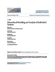
final quality of the system, it is taken at the very beginning of the development, when nothing is known in great detail. Therefore, if a wrong decision is made, that fact will be only discovered when the bottom level is reached after a lot of work was undertaken. Top-down is a suitable approach for describing something that is already clearly understood, but is not so appropriate for developing and discovering anything [Jackson, 1983, p. 370] The second obstacle is that quite often the real world does not follow a single hierarchical organization. The typical situation is to have several overlapping structures, being some of them not hierarchical: chains, networks or rings. Forcing all the structures to fit into a single hierarchy means that the system description will be distorted. A classical example of this problem is the Gregorian calendar that western countries use to measure time, since weeks do not exactly match with months. This limitation does not allow, for example, the same lower-level process to be shared by two different upper-level’s ones. As an example, consider the three DFDs shown in fig. 1(a). To maintain the single hierarchy, the designer is forced to repeat the same process (C) at the level-2 DFDs for processes A and B. This is a clumsy solution, because we are forced to remember that both C’s (1.1 and 2.3) are indeed the same. If we either write a PSPEC for that process or refine it, problems of duplication and redundancy may arise easily. One solution, depicted in fig. 1(b), for avoiding these possible problems is to rearrange some (in these case, all) of the diagrams, in order to permit processes A and B to share somehow process C. The question is that process C was “promoted” to an upper-level, which may not be correct from a pure hierarchical modeling perspective. This problem can be even quite harder to solve if the sharing processes are not at the same level. Additionally, structured methods present several limitations, whose the principal ones are [Booch, 1986]: • They do not incorporate, in a simple way, data abstraction, neither encapsulation5 . • They are inadequate for problems dealing with concurrency. • They become unstable to changes that inevitably occur during the life-cycle of any relatively complex system. 5
The word “encapsulation” is often considered to be interchangeable with “information hiding”, a concept introduced in [Parnas, 1972]. Differentiating these two terms is important since there are distinct concepts behind them. Encapsulation refers to the bundling of data with the methods that operate on that data. Often that definition is misinterpreted to mean that the data is somehow hidden. In Java, for example, we can have encapsulated data that is not hidden. Encapsulation is a language facility, whereas information hiding is a design principle.
24
t u t
1 A
w
2 B
z
t
1.1 C
u
1.2 D
v
1.3 E
w
w
2.1 F
x
2.2 G
y
2.3 C
z
z
3 C y
1 A
w
2 B
u
1.1 D
v
1.2 E
w
w
2.1 F
x
2.2 G
y
(a)
(b)
Figure 1: Promoting a process to an upper-level to reuse it.
5.3 Structured methods for real-time systems The popular appeal of the structured analysis and design methods has prompted attempts to apply their ideas to other areas, even those that do not rely upon sequential programs. This also occurred for embedded software, an area that, as already explained, as concurrency as one of its main characteristics. Several approaches, languages and tools were proposed to address the development of real-time and embedded systems, according to the principles and ideas suggested by the structured methods, namely the Design Approach for Real Time Systems (DARTS) [Gomaa, 1984] [Gomaa, 1986], the Extended System Modeling Language (ESML) [Bruyn et al., 1998], and Statemate [Harel et al., 1990], but two methods are widely considered as the most popular ones: the Ward-Mellor [Ward and Mellor, 1985] and the Hatley-Pirbhai [Hatley and Pirbhai, 1988]. The main idea of these approaches was to follow the traditional structured methods, conceived mainly to tackle information business systems, but adapt them to the peculiarities of real-time systems, where the control perspective has a major relevance. A common aspect of these methods is the introduction of state-oriented models, such as FSMs or statecharts, to specify the behavior of the control view of the system. 25
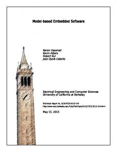
5.3.1 The Ward-Mellor method This method, also known as SA/RT (Structured Analysis for Real Time or Structured Analysis with Real-Time extensions) or RT-SA/SD (Real-Time Structured Analysis / Structured Design) is divided in two phases: the essential modeling phase and the implementation modeling phase. The essential model (a term that refers to an implementation-independent model of the system) consists of two parts: the Environmental Model and the Behavioral Model (fig. 2). The first model concentrates on defining with whom (i.e., humans and machines) the system must interact and the last one describes the required behavior of the system. Essential Model
Environmental Model
Context Diagram
Behavioral Model
Events List
Transformt. schema
Data schema
Figure 2: Ward-Mellor’s models.
The Environmental Model is used to describe the environment in which the system runs. It is composed of two modeling elements: (1) a Context Diagram, which is a description of the frontiers between the system and the external environment, indicating how both parts interface, and (2) an Events List that describes the events that take place in the environment and to which the system must react. The Behavioral Model is, as the name clearly suggests, a description of the behavior of the system. This model is also composed of two modeling elements that are informally connected: (1) a Transformation Schema [Ward, 1986] that represents, in a graphic way, the active view of the system, i.e., the layout of the transformations that operate on flows across the system boundary, and (2) a Data Schema, which denotes pictorially the structure of the data the system uses. To be clear, the Behavioral Model’s transformation schema is an extension of the DFDs proposed in [DeMarco, 1978]. Since in this report we are mainly interested in the questions that are specifically related to analysis, we do not discuss and explore the implementation modeling phase. 26
5.3.2 The Hatley-Pirbhai method This method, sometimes equally referred to as SA/RT, shares not only the alternative name6 , but also several similar ideas with the Ward-Mellor method. However, it is more elaborated in what concerns the control part of the systems being developed. It is also divided in two phases: the system specification phase and the system’s architecture definition phase. During the 1st phase, a Requirements Model is constructed, in order to characterize the system’s behavior and data flow. The requirements model is composed of a process structure, using the DFD as the main diagram, and a control structure, using Control Flow Diagrams (CFDs), a variant of DFDs, and FSMs. It is mandatory to preserve the same leveling, naming and balancing between the process structure and the control structure, and also the interconnection between both of them. In the 2nd phase, the system is partitioned into its physical components (or modules), through an Architecture Flow Diagram, which defines the modules of the system and their functional relationships and the architecture interconnection diagram that describes the way modules are interconnected.
6 DFDs In this section, we briefly describe the meta-model behind DFDs. As already stated, these diagrams were proposed in several methodologies and, as a consequence there is not a single agreed notation, neither a unique underlying metamodel. Since DFDs are not supported directly by UML, which unifies the notations proposed in several proposals, the problems solved by its creation and use still unfortunately exist for DFDs. For example, the graphical symbol for a process can be a circle [Ward and Mellor, 1985, p. 41], an ellipsis [Rumbaugh et al., 1991, p. 125] or a rectangular box [Lejk and Deeks, 2002, p. 64]. Although these are problems at the syntactic level, they nevertheless do not facilitate the immediate understanding of a description and were responsible for the almost null communication amongst computer tools of different vendors.
6.1 Data-flow paradigm of computation As a modeling technique, DFDs belong to the family of languages included in the data-flow paradigm. Under this paradigm, computation is described as a directed graph, where the nodes represent processes (or functions) and the arcs represent data paths. The data-flow principle is that a node can perform its operations whenever input data are available on the respective incoming arcs. Thus, several 6
For more details on the method’s name, please refer to [Hatley et al., 2000, pp. 5–6].
27
nodes may execute simultaneously and hence the concurrency is inherent to this paradigm. Data-flow programs are said to be data-driven or data-trigger, because their execution is determined by the availability of data to be processed. Even though, in this report, we mainly concentrate on the DFD, several other meta-models exist that can be included in the data-flow paradigm, namely, Kahn Process Networks (KPNs) [Kahn, 1974], Flow Graphs [Aho et al., 1986, pp. 532– 4], Data-Flow Process Networks (DPNs) [Lee and Parks, 1995], Flow Diagrams [Böhm and Jacopini, 1966], Computation Graphs [Karp and Miller, 1966], Synchronous Data-Flow (SDF) Graphs [Lee and Messerschmitt, 1987], and Petri Nets (PNs) [Murata, 1989]. There are some semantical differences among these modeling languages, but they also share a lot of similarities; for example, DPNs are a special case of KPNs [Edwards et al., 1997] [Lee and Parks, 1995] and Computation Graphs have been shown to be a special case of Petri Nets [Peterson, 1977] [Peterson, 1981, pp. 213–6]. Some graphical data-flow tools are also available for the development of signal and image processing systems, namely Khoros, Ptolemy and LabVIEW. In the area of embedded systems, traditionally connected to the electrical engineering field, the designation “graph” is much more popular than “diagram”, which appears to be the most preferred term in the software engineering community. For more details on data-flow languages, namely an historical retrospective, the interested reader is referred to [Whiting and Pascoe, 1994].
A historical note on DFDs The DFD was introduced in the structured design to represent the data entities and the processes that transform them [Stevens et al., 1974] [Yourdon and Constantine, 1978]. DFDs and other diagrams were used to promoting programming languages concepts into modelinglevel ones, based on pictorial representations. The program was regarded as having a pipe-and-filter architecture, which provides a structure for systems that process a stream of data: each processing step is encapsulated in a filter component and data is passed through pipes between adjacent filters [Buschmann et al., 1996, p. 53]. The DFD ‘bubbles’ were the filters and the architecture was then implemented as a procedure hierarchy.
DFDs, as originally proposed by De Marco, Yourdon and others, were good at describing the flow of data among pieces of functionality, but they were not so effective at showing the control perspective of the system. A DFD does not show control information, such as the time at which the processes are executed 28
or decisions in relation to alternate paths. This information belongs to the dynamic model of the system. These limitation were partially remedied in WardMellor and Hatley-Pirbhai methods, which are more adequate for control-oriented applications. Ward-Mellor’s extended DFDs constitute indeed an heterogeneous meta-model, since they incorporate in the same notation both an activity-oriented perspective and a control-oriented perspective. Here we follow the specific DFDs proposed in the Ward-Mellor method, since it is considered, as already mentioned, an emblematic example of a structured analysis and design method for complex systems, namely real-time ones. The reader is referred to chapter 6 of their book [Ward and Mellor, 1985] to further details on their DFD notation and corresponding meta-model.
6.2 Ward-Mellor’s DFDs DFDs use four symbols to represent any system at any level of detail. The four modeling concepts that must be represented are: data flows (movement of data in the system), data stores (repositories for data that is not moving), processes (transformation of incoming data flows into outgoing data flows), and external entities (sources or destinations outside the specified system boundary, also known as terminals). The main element of a DFD is the transformation that is depicted by a circle. Transformations, the term used within the Ward-Mellor method, represent processes, and from herein we will use both designations interchangeably. In computer jargon, processes are also designated as ‘bubbles’ due to their circular aspect. The processes can be connected by labeled flows (input, output, and input/output). An example of a system that produces an encoded message from a plain-text one is shown in fig. 3. Plain message
Code
1 Encode Message
Encoded message
Figure 3: An example of a small DFD.
Processes are supposed to execute instantaneously. The processes depicted in a DFD are, at least potentially, concurrent, which means that no sequencing is implied. However, since there are flows connecting the processes, a causality relation may exist among processes. If the output flow of one process is also the 29
input flow of another process, the two processes are in a sequence (fig. 4 shows an example). Each process is assigned a number, but the first numbered process need not occur before the second one, although it may. This implies that exchanging the numbers of the processes in fig. 4 was possible, but the chosen numbering is preferable since it clarifies the meaning of the diagram. Each process in a DFD can be decomposed into a new DFD, which is to be understood as the child of the decomposed process. This is to be viewed in the same way as a routine can be decomposed into lower level ones. This decomposition of processes continues until a level, at which the processes can be easily described, is reached. These latter processes are called functional primitives and are described, traditionally, with a PSPEC (Process Specification). PSPECs specify concisely and briefly, according to the structured methods’ proponents, the intended behavior, in a natural language, eventually complemented with equations, tables and diagrams. As a rule of thumb, a PSPEC is usually less than one page long, but sometimes is only a few lines long. This depends on the granularity for primitive processes and on the level of detail for the specification. Receiver's email address Plain message
Code
1 Encode Message
Encoded message
2 Send Email
Email message
Figure 4: Processes of a DFD in sequence.
Another important concept associated with DFDs is the data store. The store represents an item or a set of them that is transformed by processes, but whose basic nature remains unchanged. The data store is represented by two parallel line segments with the name of the store written between them. Stores and transformations can be interconnected, but the flows among them are not labeled. The arrow heads that can be added at the ends of the flows have the following meaning: • An arrow head pointing from a store to a process means that some output flow of the process uses some data from the store. • An arrow head pointing from a process to a store means that the store is changed in value or in set membership by the process. 30
• A bi-directional arrow between a process and a store means that both previous characteristics apply. It can be seen as a compact notation for two uni-directional flows, one in each direction. An example of a DFD with a data store, representing a CRUD7 application, is presented in fig. 5. The data flows connect the external entities to processes or one process to another one. A data flow is represented as an arrow between the producer and the consumer of the data value. A description of the data, usually its name and/or type, labels the flow. The same value can be sent simultaneously to more than one consumer. This is drawn as a fork with various arrows departing from it. The arrow parts after the fork point are not labeled, since they represent the same value that appears in the common part of the flow. There is also the possibility of splitting a structured value (like a record or an array) into its components, each one being sent to different destinations. Customer Information
Account Number
Account Number
1 Create Account
Account Status
2 Read Account
Bank Account
3 Update Account
4 Delete Account
Account Number Account Number
Movement
Figure 5: A DFD with a data store.
The flows can be divided into three main categories, as indicated in fig. 6. 7
CRUD is an acronym for “Create, Read, Update, Delete” and it refers to the typical operations that exist to manipulate records of data in a database application.
31
Type of flow
Symbol
Time-discrete flow Time-continuous flow Event
Figure 6: DFD flows.
A time-discrete flow, also designated as a time-transient flow, exists or provides values only at individual moments in time. Thus, it is considered to have an undefined or null value at all other times. A time-discrete flow is roughly equivalent to the idea of a transaction, as used in information systems terminology. This type of flow represents both the occurrence of the flow and the respective data. In contrast, a time-continuous flow is useful to represent characteristics of the physical world, such as a temperature, a pressure or a voltage. It represents an entity that exists at every instant within a time interval, such as a variable that changes its value according to a continuous function of time. An event is used to represent signals that indicate that something has happened. In a sense, there is no content associated to events. A process that only handles, as inputs and outputs, events is called a control transformation (or control process). Analogously, an event store (a data store for events) can also be used to record occurrences of events. An example involving one event store and one control process is presented in fig. 7. The events that flow from control processes to data transformations are to be understood as prompts or triggers, i.e., they simply switch on or off the data transformations. The DFD notation also includes the possibility of compactly specifying multiple instances of the same basic model. The convention is to use a double circle to denote multiple instances of the same (control or data) process. An example of this notation is shown in fig. 8.
6.3
Some problems and limitations of DFDs
DFDs seem to have certain advantages over other modeling techniques. First of all, they are well-known by almost all computing professionals: in 1996 DFDs were the most popular tool taught in systems analysis and design courses in universities across the USA: 597 out of 647 schools (92%) indicated that they taught DFDs in that course [McLeod Jr., 1996]. Although this is not a technical argu32
Output Valve Closed
Valve Status
Control Vessel
Start
Open Input Valve
Stop
Figure 7: A DFD with an event store and a control process.
Output Valve Closed
Valve Status
Start
Control Vessel
Open Input Valve
Stop
Figure 8: A DFD with multiple instances of the same control process.
33
ment and even admitting that nowadays this figure may be different (i.e., smaller), in any case it represents that technical people are able to read DFDs. Secondly, it has been showed that DFDs produce higher-quality solutions in process-oriented tasks and are not inferior to object-oriented methodologies even in object-oriented tasks [Agarwal et al., 1996]. In addition, empirical research also confirmed that DFDs are easier to learn and to use [Yadav et al., 1988] [Vessey and Conger, 1994] [Moynihan, 1996]. Despite these strong points in favor of DFDs, they also have several limitations and semantical divergences among the several different proposals, which are important to identify and explain in this report. In DFDs, the data flows from one process to another and then stops in a data store (also known as data repository or, simply, file). According to some authors, the user seems to be confused by these diagrams because the line between system and user responsibility is not evident [Kulak and Guiney, 2000, p. 20]. Furthermore, a DFD contains usually more details than those users are prepared to deal with; for example, the number of data repositories and what they store is a problem that typically does not concern users. Our belief is that DFDs should not be used for capturing the user’s requirements, but that they are still useful in subsequent phases of the development, especially for embedded systems, which emphasize predominantly the behavioral or dynamic part of the system. In fact there are data-intensive and signal processing embedded systems, where the data being operated has a great importance and hence must be carefully modeled. This situation contrasts with control-oriented embedded systems, where the most important aspect is the behavior. We will come back to DFDs, namely in section 6, since the main aim of this report is to analyze how to combine the functional and the object-oriented views and DFDs do constitute one of the main meta-models that are used to express the functional views of the systems. One problem related with the symbol for a DFD process is that it represents something very general [Jackson, 1995, p. 48]. This problem does not exist, for example, in the discipline of digital systems, where each symbol, a OR2 gate, for example, has a more precise meaning, at least at some level of abstraction. We know what happens to the OR2 gate’s output for every combination of the binary inputs and, more importantly, we can calculate what is the expected behavior of a diagram composed of several connected gates. A process in a DFD can represent either a passive or active transformation; it also does not show how the inputs relate to the outputs; and it can represent either a process that executes continuously or only at discrete points in time. Since the meaning of a process is so vague, namely when the development is in its beginnings, usually its name and the labels of the flows connected to it carry all the responsibility for describing the intended behavior. 34
Yet another problem is concerned with the fact that a set of DFDs is to be viewed as a model of the requirements of a system, not a representation of the system’s implementation [Hatley and Pirbhai, 1988, p. 55]. This model is very idealized in the sense that it assumes to be triggered by data and to execute hugely fast, i.e., instantaneously. This contrasts with the implementation which probably will not be data-triggered and will surely takes time to execute. The DFDs do not assume that the processes will run sequentially or in parallel: processes can run in parallel as long as they have data available. If the implementation imposes sequential processing, this is to be seen as a constraint of the platform, not the model. DFDs do not have a unique semantics, since they differ according to the interests of their proponents and the characteristics of the application domain. In this report we just examine some of those semantical discrepancies on the DFDs proposed by Ward-Mellor against those suggested by Hatley-Pirbhai. The processes are supposed to be triggered by data: whenever there are sufficient input data, the process performs its transformation. However, according to Ward-Mellor, this just happens if there are no events connected to the process. If input events exist, the process executes only when the process is enabled and input data exist; if the process is disabled, input data is simply discarded [Ward and Mellor, 1985, pp. 94–5]. This implies that the processes themselves have memory, since they are activated and deactivated by switching them on and off, respectively. Hatley-Pirbhai follows a distinct approach. Processes are executed when: (1) data are available at its input flows; (2) activation conditions are met (example, process is idle); and (3) internal timing requirements are satisfied (example, every 30 seconds) [Baresi and Pezzè, 1998]. In any case, processes are not procedures with a call-return semantics. Another semantical question that must be clarified is what happens to a process with at least one time-continuous input flow. Since data are always available, the process must in principle execute continuously. In Ward-Mellor, the process, if enabled, may begin producing values on the output flows; if the process is disabled, no output flows can be generated [Ward and Mellor, 1985, pp. 96]. In HatleyPirbhai, it is not mandatory for a process to be triggered by discrete flows. Thus, since values on time-continuous flows are always available, processes with them as inputs can either execute continuously or only when there is a modification on the value [Baresi and Pezzè, 1998]. This choice seems to have some implications, not only in terms of performance, but also in what concerns the number of times the adjacent processes have to execute. These examples show that it is possible to associate different semantics to DFDs. 35
7
UML
In this section, we discuss the use of graphical notations by software development methods, namely UML. We also present some arguments to justify the noninclusion of DFDs in UML and describe the typical usage of the UML diagrams, during the analysis of a system.
7.1
Graphical notations
One common aspect of structured and object-oriented methods is that they usually adopt graphical notations for describing the system under analysis. For a graphical notation to be useful it must be clear and intuitive, so that both clients and designers can understand them, but also precise and rigorous, so that computer tools can analyze, simulate and validate them [Harel, 1988]. One drawback of graphical representations is that they are not adequate for capturing detail. A graphical model that has excessive information becomes as hard to read as an equivalent textual description. One of the languages that is gaining exponential popularity and usage is the Unified Modeling Language (UML). UML is a graphical modeling language, that supposedly unifies and integrates the different notations used before by the numerous methodologies proposed. This notation became a real necessity, because, between 1989 and 1994, the number of object-oriented methods increased from fewer than 10 to more than 50 [Booch, 1999]. UML constitutes the de facto standard notation and semantics for properly describing software built with objectoriented or component-based technology. It is undoubtedly a step in the right direction, but it is not a perfect or universal modeling language [Engels et al., 2000]. We believe that UML, as it stands today, must be, in some contexts and for some application domains, complemented with other meta-models or at least adapted (by stereotyping it) to address those meta-models. As an example, for modeling the behavior of the system’ components that have a complex or interesting dynamic behaviour, a state-oriented model can be specified. UML has two different meta-models for this purpose: statecharts and activity diagrams. These two meta-models present many important characteristics for reactive systems, namely concurrency and hierarchy, but they do not allow an elegant treatment of the data path/plant resources and the specification of dynamic parallelism. These are two crucial necessities for embedded software, since different parts of the system may try to access simultaneously the same resources. Thus, we believe that for control embedded systems, the usage of Petri nets (PNs) in conjunction with other UML models can give good results [Machado et al., 2001] [Jørgensen and Christensen, 2002]. Although we do not explore this topic in this article, the usage of PNs, namely their high36
level variants, is considered a proper technique to give a formal flavor to DFDs [Tse and Pong, 1989] [Elmstrøm et al., 1993]. Henceforth, combining UML with PNs could also be seen as a solution to the problem being addressed in this report. Another problem with UML is that its semantics is not precise or rigorous. This is a recurring problem of graphical notations, since they seem to carry a higher risk of vagueness than textual languages [Harel and Rumpe, 2000]; for instance, lines and boxes suggest less need of preciseness than identifiers and assignment statements [Jackson, 1995, p. 91]. The reason for this to happen is that graphical languages are typically used without a compiler (i.e., a computer tool that would inform, at least, if the described model is syntactically correct). Although this can also occur with textual languages (we can use a simple text editor to write the program), it is more frequent to process them with compilers. Therefore, the exclusive use of graphically-based and intuitive notations is often insufficient for correctly specifying a given system. Since UML is a multiple-view meta-model, a serious consequence is that inconsistencies, among the diagrams used for specifying the system, may occur. This also happens when the designers are using computer tools for editing the diagrams, since usually those tools do not perform all kinds of checks necessary to guarantee full consistency. In large projects, where it is common to have several team members modifying the same set of diagrams, consistency is even more difficult to guarantee. Several attempts have been made to remedy this problem [Krishnan, 2000] [Küster and Stroop, 2001] [Derrick et al., 2002], because it usually proves to be costly in software development projects.
7.2 Why UML does not include DFDs? In this context, we would like to answer in this report the following question: “why DFDs were not included in UML?” This is a quite intriguing question for us, since OMT, a methodology devised by a team headed by James Rumbaugh, one of the leaders of the UML movement, includes DFDs as one of its diagrams [Rumbaugh et al., 1991]. In our opinion, the answer to this question can be found in a combination of the following four arguments: 1. UML was created mainly with the ideas and concepts from the OOSE, OMT-2, and Booch methods. OMT-2 was a revision of OMT with the formal introduction of use cases into the methodology [Rumbaugh, 1994]. OMT-2 has special expressiveness for analysis and data-intensive information systems [Booch, 1999] and since that special type of systems have usually a trivial functional model [Rumbaugh et al., 1991, p. 123], it is easy to understand the non-inclusion of DFDs within UML. 37
2. Although useful for different development purposes, DFDs conflict somehow with the spirit of object-orientation. 3. Within OMT, classes and DFDs are developed in parallel and only later are they associated. The consequence is that this association is not properly integrated and is quite difficult to establish, which means that the approach is not intuitive and easy to apply in the general case [Rumpe et al., 1999]. 4. UML was conceived as a general-purpose modeling language for objectoriented software systems [Selic et al., 2002]. DFDs got some bad reputation within the software engineering community, when structured methods were considered old-fashioned and object-oriented become the new ‘silver bullet’. So, the inclusion of DFDs into UML would be regarded as not attractive, especially from a commercial or marketing point of view, despite the fact that there are not too many strong technical arguments for not supporting it. We are specifically interested in understanding how DFDs can be combined with other UML diagrams, in order to model embedded software. We have strong intuitions that DFDs are valuable models, especially for embedded software, and we would like to investigate how they can be gracefully combined with UML to model this type of software.
7.3
Typical usage of UML
The most common way to use UML diagrams during analysis is to start with use case diagrams and to proceed with sequence diagrams, in order to describe some scenarios of the communication of the system with its actors. Later, a class diagram is created, taken into consideration the previous diagrams. Usually a state-chart diagram is associated to each class for describing the corresponding behavior. Although UML includes nine diagrams, using only the referred four during analysis seems to be sufficient for the majority of developers [Douglass, 2000] [Howerton and Hinchey, 2000] [Jigorea et al., 2000] [McKinley et al., 2001]. In fact, collaboration diagrams are not included, because they are similar to sequence diagrams, activity diagrams are usually ignored, since they represent a subset of statechart diagrams and component and deployment are not at all used or only used in later development stages [Porres, 2001, p. 54]. We find two major problems with this typical usage, in what concerns the development of an embedded system. Firstly, the “jump” from use cases and scenarios to classes is, in our opinion, a very big one. This step requires too much ingenuity and there is not an evident direct relationship between use cases and 38
classes. We think that there exist many similarities between this transformation step and the transition from analysis to design in structured methods, which was vastly criticized to be one of the biggest limitations of those methods. Instead, what we need to develop complex embedded systems is a seamless process, from requirements until the coding phase, that preserves the behavior and integrity of the models in each development step [Pnueli, 2002]. Secondly, for embedded software, we think that the attention should be focused towards object diagrams, instead of class diagrams. The majority of the methodologies for developing software do not pay too much attention to the object diagram. In fact, software developers concentrate too much on the class structure and too little on the object structure [Sigfried, 1996, p. 146]. Finally, it is important to discuss what are the most typical mistakes that prevent organizations to get more value from using UML in their software development projects [Booch, 2002]. Firstly, it is crucial that the UML models do not possess a level of detail similar to the final executing system. Models are abstractions of the reality and serve “only” to visualize, specify, document the software. Therefore, producing quality executable programs is, almost always, the main aim of any project8 . Secondly, some companies utilize UML just as a documentation notation. This is a very limited way of taking advantage from UML, since using it as a communication medium among the various stakeholders proves usually useful. Thirdly, it is important that every developer should use and understand UML to get the most value from it. If programmers (i.e., the developers that actually write the final code) do not strongly rely on the UML models to construct the system, then big mismatches between the UML models (that represent the user’s and system’s requirements) and the final system will arise easily and naturally.
7.4 Classes vs. objects The typical focus towards classes may be caused by the fact that many software engineers still do not clearly distinguish between objects and classes [Meyer, 1988, p. 52] [Szyperski, 1998, p. 8]. This confusion is greatly related to the intangible nature of software. Building models that simultaneously have objects and classes should not be endorsed for two main reasons. Firstly, a class may be viewed as a pattern that allows the creation of objects for the application under development, but also for future applications. Secondly, objects represent the elements that do constitute the application. Therefore, taken into account this perspective, the authors strongly recommend, as a guideline for system’s development, that 8
The automatic generation of executable code (or a program in a high-level programming language) from models specified in a modeling language, such as UML, is not yet fully realized, but it is not difficult to predict that, in the near future, it will be a reality. Achieving this aim is the main purpose of the OMG’s Model-Driven Architecture (MDA) initiative [Bézivin, 2001].
39
it is preferable to not incorporate simultaneously classes and objects in the same model or diagram. For conventional software, the class diagram is built firstly, but we believe that for embedded software, that order must be reversed. To develop embedded software, it is more important to have a good object model than a good class diagram, because the elements that do constitute the system are the objects and not their classes. Obviously, the best situation is having good object diagrams and good class diagrams. We are not suggesting to roughly treat the class diagram or even to ignore it, but to focus the attention towards the construction of the object diagram. This is the main reason for us to recommend, when developing embedded systems, to first identify the objects and to later select the classes to which those objects belong. The object model defines the structure or the architecture of the system by describing the objects of the problem domain and their relationships [Kuusela, 1998]. The architecture of the software refers to the essential structural and behavioral framework, on which all other aspects of the system can be built upon. A welldesigned architecture simplifies the construction of the application, but allows also its evolution, which is a topic of great interest for complex systems [Selic, 1998]. The emphasis on objects (instances) is justified by the fact that we are dealing with real-time embedded systems. This object-driven or component-based approach is typically followed for developing control-oriented systems, where the final architecture and the concepts of abstraction and modularity are key topics to guarantee that the non-functional requirements (heterogeneity, ubiquity, faulttolerance, security, dependability) are met. In contrast, class-driven approaches are used for information-intensive applications, such as databases, where the relations among classes (types) and its hierarchical categorization are the most important issues to take into account. This perspective that puts classes in an apparently secondary role may be classified by some specialists as object-based rather than object-oriented. However, the approach that firstly defines the objects and later the classes is somehow consistent with the bottom-up discovery of inheritance to organize the classes [Rumbaugh et al., 1991, p. 163]. During the classification of objects the class structure is built, modified, or ideally just (re)used. Reuse can be achieved in 3 different ways, during the classes discovery. First, if there are more than one object of the same class, their definition is specified in just one place. Second, if classes with similar properties are found, hierarchical relations among those classes can be defined. Finally, when a class is being described, the developer can recognize the existence of that class in a library, which allows it to be immediately reused. The class diagram is usually understood as a template for a set of applications that can be obtained from it. In other words, the class diagram is a high-level gen40
eralization of the system [Lyons, 1998]. When developers define the way classes are interrelated, they are indicating all the systems (or all the configurations) that can be obtained from those classes. With this perspective, it is common not to build the object diagram, since it can be automatically derived from the class diagram. In the cases where an object diagram is built, it is mandatory to guarantee that the relations expressed in the class diagram between two classes also exist between instances of those classes. This is the main reason why methodologies usually suggest class diagrams to be first elaborated than object diagrams. This implies an additional task in which it must be assured that there is consistency between the information that is described by both diagrams [Douglass, 1998, p. 130]. This fact means that some information is being unnecessarily replicated. For instance, the existence of the «singleton» stereotype in UML, which indicates that a given class can only have one instance, corroborates the perspective that sees the class diagram as a pattern for the systems, within a given application domain. This stereotype clearly indicates that if the object diagram is to be made consistent with the class diagram, it must satisfy the restriction of just presenting one single instance of that singleton class. The class-centered approach seems adequate to develop business information systems or, more generally, any data-dominated system, where the objects are created and destroyed during the system life cycle. For example, in a system for bank accounts management, it is common that each account is always associated with, at least, one customer. This fact is indicated in the class diagram by associating the account class with the customer class. When an account object is created, it must be linked to, at least, one customer object. This approach does not offer many benefits for developing embedded systems, since normally the objects that constitute the system are not created and destroyed on the fly. Actually, structure is one of the dominant aspects of real-time and embedded systems [Selic, 1999]. An embedded system is generally composed of a set of fixed objects that are linked in some way and this organization can be perfectly described by an object or a collaboration diagram. Thus, it is not crucial to indicate, for example, that objects of the controller class need to be linked with objects of the sensor class, because this fact is not at all universal. If in some applications this information can be important, it may completely wrong in others. As already stated in this report, another important concern related to embedded software is the description of concurrency. The notion of concurrency can also be modeled in UML using objects, namely active ones [Selic, 1999] [Porres, 2001, p. 108]. An active object is continuously executing, which requires its own thread of control, and runs concurrently with other active objects. The ‘Embedded UML’ profile proposes also the concept of a reactive object, which consists of a concurrent process, with asynchronous communications to other objects, that reacts to 41
external events and stimuli [Martin et al., 2001]. A reactive class is one that can react to events and, therefore, must specify a control structure, typically in the form of a state-oriented model, and communication with other objects through ports and connectors, which gives raise to collaboration diagrams. So, objects do play a fundamental role in modeling embedded software systems. Additionally, objects, if viewed as components, could also encourage the adoption of component-based software development, which promotes the creation of complex system by connecting off-the-shelf building blocks. Even though there are some component-based proposals for embedded software [Urting et al., 2002] [Genßler et al., 2002], this kind of development in this computer field is not yet as popular as expected to be, because critical issues, such as size, performance, power and cost, are not usually considered by the component-based methodologies [Friedrich et al., 2001].
8
Our proposals for combining DFDs with UML
In this section, we present some proposals to combine DFDs with other UML models within the development of embedded software. It is essential to observe that we are not able to claim undoubtedly that our proposals can help the designers, although we have some intuitions that they do. In fact, measuring the utility of a technique, method or approach is not simple, whatever the chosen angle. The software practitioners are, in our opinion, the real and final judges of theses ideas: if they are applied, there must be some value and utility on them; if not, they are just academic work with no real practical value. But before presenting our ideas, we first review some of the proposals made by other researchers on the more general problem of combining the functional approach with the object-oriented one.
8.1
Related work on DFDs and objects
Some authors have already experienced the inclusion of DFDs with object-oriented methods. In one proposal [Wang and Cheng, 1998], the DFD notation is modified and the role of the functional models are redefined, in order to use DFDs while retaining the spirit of object-orientation. Two types of functional models are suggested: Object Functional Models (OFM) and Service Refinement Functional Models (SRFM). OFMs are used to model the services provided by individual objects, while SFRMs model how the services of individual objects can be composed to implement the services of their corresponding aggregation object. In both models, the only modeling elements are: objects, processes and data-flows. The data store is not necessary, according to the authors, since they use an object for that 42
purpose. The interactions with a data store are modeled as communications with the corresponding object. In another proposal [Becker et al., 2000], the functionality associated with each use case is described as an E-DFD (an extended version of the traditional DFD). A tool, called SysObj, uses these diagrams as inputs to automatically generate an object model, that is viewed as the architecture of the system. This method is also related to an integrated environment for developing distributed systems with the object-oriented paradigm [Becker et al., 1999]. In OMT, DFDs are also used to describe the functional model of a system. Since in OMT the system is also specified by two other models (the object and the dynamic models), DFDs specify the meaning of the operations in the object model and the actions in the dynamic model [Rumbaugh et al., 1991, p. 123]. Although there is some attempt at integration, this correspondence is left completely vague and can not be analyzed in any useful way. For reverse engineering purposes, the adoption of reverse generated DFDs (i.e., DFDs obtained after reading and interpreting the source code) is proposed as the basis to obtain the objects that a system is composed of [Gall and Klösch, 1995]. The approach is said to be hybrid, because it is not fully automatic, requiring in specific occasions the assistance of a human expert with knowledge of the domain. Again for reverse engineering, the combined usage of DFDs and ERDs is suggested to describe the system being modernized [Jacobson and Lindström, 1991]. Alabiso also proposes the transformation of DFDs into objects [Alabiso, 1988]. In order to accomplish the transformation, he proposes the following four activities: 1. Interpret Data, Data Processes, Data Stores and External Entities in terms of object-oriented concepts. 2. Interpret the DFD hierarchy in terms of object decomposition. 3. Interpret the meaning of Control Processes for the object-oriented model. 4. Use data decomposition to guide the definition of the object decomposition. Within the Object-Process Methodology (OPM), the combined usage of objects and processes is recommended [Dori, 2002a]. An Object-Process Diagram (OPD) can include both processes and objects, which are viewed as complementary entities that together describe the structure and behavior of the system [Peleg and Dori, 1998]. Objects are persistent entities and processes transform the objects by generating, consuming or affecting them. In addition, states are also integrated in OPDs to describe the objects. The usage of OPM, for modeling, specifying, and designing reactive and real-time systems, was also proposed, by 43
extending the notation with notions such as timing constraints, events, conditions, exceptions, and control flow constructs [Peleg and Dori, 1999]. Another interesting proposal is the Functional and Object-Oriented Methodology (FOOM) [Shoval and Kabeli, 2001], which is specifically tailored for information systems. The main idea behind FOOM is to use the functional approach, at the analysis phase, to define users’ requirements and the object-oriented approach, at the design phase, to specify the structure and behavior of the system. In the FOOM, the specification of the user’s requirements is accomplished, in functional terms, by OO-DFDs (a DFD with data stores replaced by classes), and in data terms by an initial object-oriented schema, or an ERD which is easily transformed into an initial object-oriented schema. In the design phase, the artifacts from the analysis are used to create detailed object-oriented and behavior schemas. These schemas are the input to the implementation phase, where an object-oriented programming language is adopted to create an executable program for the system at hand.
8.2
Global context
In our opinion, the combined usage of DFDs with other UML models can be accomplished in several ways and this combination must be interpreted in a very broad sense. This results from the fact that the development of a software system proceeds in steps, where several different models are being refined and detailed, but also transformed, merged, split, integrated, etc. Therefore, in this context, the term “combined” used above can mean several different things. One possibility is that DFDs are used during the development process and that they are transformed into UML diagrams or vice versa. A distinct interpretation consists in not using DFDs at all, and give some UML diagram a DFD flavor. Another possible alternative is to use DFDs and UML diagrams, and propose techniques for integrating their usage. Under these circumstances, the question that is important to answer is how and when can DFDs be used within the development process of an embedded system. The way to tackle this question can be divided in three more specific ones, to which we hope to give real answers in this report: 1. Are DFDs an useful model for embedded software? 2. In which phase of the development process must DFDs be introduced? 3. Which views should DFDs cover? We do think that DFDs can be, in some contexts, an useful model for embedded software. This idea can be largely confirmed by the widespread usage 44
of data-flow oriented meta-models for describing digital and embedded systems, namely Process Networks [Lee and Parks, 1995] [Kienhuis et al., 2000] and Control/Data Flow Graphs [Gajski et al., 1992, p. 139] [Gajski et al., 1994, pp. 36–9] [Middelhoek and Rajan, 1996] [Wolf, 2000, pp. 254–7]. It is important to stress that the meta-model behind CDFG has many resemblances to the one associated with DFDs with control extensions (as proposed in the Ward-Mellor method, for example). However, for developing embedded software, we do not believe that it is possible to rely on a “one-size-fits-all” solution, due to the wide range of applications covered by this software field, as discussed in section 2. This means that in some situations DFDs may be an adequate model of computation, but that in others they may not. As already stated, we think that a data-flow model may be the most adequate one for transformational systems, that is, systems that continuously repeat the same data transformation on streams of data [Gajski and Vahid, 1995]. Application areas, where the data-flow paradigm of computation is evidently useful and widely adopted, include for example multimedia systems [Masselos et al., 1999] [Yang et al., 2002], telecommunication devices [Helm and Wess, 1996], and digital signal-processing systems [Bhattacharyya et al., 1996] [Benini et al., 2000]. Furthermore, DFDs are also very good at producing systems based on a menu structure, because the idea of functional decomposition and leveling is just right for a menu-based development [Lejk and Deeks, 2002, p. 252]. The incorporation of DFDs into UML can not be made without first deciding if they are merely added as a new diagram or whether it is convenient and possible to view them as an extension or adaptation of an already existing UML diagram. The combined use of DFDs with other UML models, if deemed useful, can be accomplished with at least two approaches, whose differences are depicted in fig. 9. In the first alternative, shown in fig. 9(a), the DFD meta-model is mapped into UML concepts, while in the second one, shown in fig. 9(b), both meta-models (UML’s and DFD’s) are available as originally devised. We think that the first alternative is preferable, because it allows us to restrict to the UML meta-model in what concerns the model’s back-end processing (model transformation, validation, code generation). This restriction allows the usage, without any modification, of any tool that supports UML for edition, documentation, validation, simulation and code generation purposes. It also permits, for example, the direct usage of the formalization of UML with Rialto (previously designated SMDL) [Björklund and Lilius, 2002]. However, this solution forces the DFDs to be adapted to a given UML diagram, which means that probably we are not able to use DFDs at their maximum expressive power. Another argument in favor of the first alternative is that almost all people involved in UML agree that it already offers a reasonable number of modeling diagrams, sufficient for the vast majority of modeling purposes, and that it should not be further extended, namely 45
DFD
UML
DFD
back-end procesing tools
UML
back-end procesing tools
(a)
(b)
Figure 9: Two alternatives for integrating DFDs in UML: (a) DFDs mapped into UML concepts; (b) DFDs added to the UML meta-model.
in what concerns the number of diagrams [Rumpe et al., 1999] [Selic et al., 2002] [Dori, 2002b]. In any case, to take full advantages of DFDs, the designer must be completely aware of their associated meta-model. So, even in the situation where a UML diagram is adapted to be viewed as a DFD, the designers have to understand the complete set UML+DFD. Under this assumption, the argument that in this case adapting a UML diagram may result in confusion and misunderstandings is not a valid one for us. We propose three major ways of using, in an integrated way, DFDs within an object-oriented system development. 1. DFDs to refine the use case model; 2. DFDs to detail the behavior of a system’s component; 3. DFDs to be transformed into class diagrams. The rationale behind these proposals is always to have, as the major model to drive the implementation phase, some object or class diagram, so that an objectoriented programming languages can be used, but also to include the DFDs in the modeling process.
8.3
DFDs to refine the use case model
8.3.1 Initial considerations It is commonly accepted, within the object-oriented community, that the analysis of a software system should be started with uses cases. A use case diagram represents a functional view of the system. Similarly, in structured methods, a system is 46
seen as a provider of functions to the user, which was already stated in this report to be an adequate view for requirements capture. However, using use cases does not necessarily implies that subsequently an object-oriented approach must be followed. Use cases represent a technique that is quite independent of object-oriented modeling and can be applied to any system, developed either with a structured or object-oriented approach [Jacobson, 1994]. In any case, adopting use case diagrams should not be seen as an opportunity to follow again a functional decomposition of the system. This is the reason for our proposals to incorporate always object-oriented diagrams in the modeling process. In this context, it seems that the transformation of a use case model into a DFD-like model is not at all awkward or forced, since both meta-models can be used naturally for focusing on the same modeling perspective. DFDs can be made more detailed, since they include processes (similar concept to use cases) and external entities (identical to actors in use case models), but also data stores and data flows, which indicate data-dependencies among processes and are not directly representable in a use case diagram. Even though UML provides two relationships, «include» and «extend», to connect use cases among them, they are not related to data or control flows, but rather with dependencies between use cases. We will not explore further this topic, since the relationships seem to confuse, instead of helping, the designers [Génova et al., 2002]. Therefore, we do not suggest their usage in the diagrams. If the diagrams that describe the same system, depicted in figs. 5 and 10, are compared, we clearly notice that DFDs are more detailed than use cases. As a matter of fact, it is usually difficult to perceive how use cases interact, especially whenever there are many of them in a diagram. An interesting solution to this limitation is to use an activity diagram that shows how use cases are related and also alternatives and decisions [Mellor and Balcer, 2002, p. 51]. As already stated before, we would like, if possible, to use UML as the notation to represent the systems being modeled. Therefore, the meta-model behind DFDs must somehow be mapped into UML concepts. Generically speaking, any UML diagram could be used for this purpose, as long as stereotypes are associated to its constructs. In the extreme case, we were only using the syntax of the diagrams, but would associate a very different semantics to it. But we prefer to adapt a UML diagram whose respective model of computation is as close as possible to DFD’s one. However, this choice should be taken with care, since different diagrammatic representations do not necessarily have the same effectiveness or computational power [Hahn and Kim, 1999]. Before choosing which UML diagrams best match with DFDs, it is important to notice that DFDs are not representing only the behavior of the system. We can also think about DFDs as defining a given structure or architecture for the application being analyzed: they are dividing or decomposing it in its modules or 47
bank clerk
costumer
Create Account
Read Account
Update Account
Delete Account
Figure 10: A use case diagram for a CRUD application.
subsystems and also showing the communication paths amongst those modules. As a matter of fact, DFDs can be used to describe only the structure of a system, showing just its components and the channels through which information flows [Harel and Rumpe, 2000]. With this view on DFDs, no behavioral aspect is being modeled. In the case of DFDs, the behavior is usually organized as a tree of processes and only the leaf ones (also called functional primitives) must be associated with a description, traditionally a PSPEC (Process Specification), that specifies concisely and briefly the intended behavior. In fact, when a system is divided in parts both structure and behavior are being decomposed. For example, some authors consider that the design methods that have evolved to work with object-oriented, procedural and functional languages all tend to break the systems down into units of behavior [Kiczales et al., 1997]. They consider that all systems are submitted to a functional decomposition, even if, for each computational paradigm, different units of behavior (objects, procedures, and functions) are considered. Similarly, it seems thus acceptable that we consider that all those design methods force equally the systems to a structural decomposition. 8.3.2
Selection of a UML diagram to represent DFDs
Taking into account that it is acceptable to view DFDs as a structural notation, we had considered initially the following UML diagrams as possible solutions to represent DFDs: object diagrams, collaboration diagrams, component diagrams, deployment diagrams, and activity diagrams. Despite the fact that class diagrams 48
constitute also a static model, they are not considered here as a primary option, due to the reasons pointed out in subsection 7.4. Component diagrams and deployment diagrams were rejected from the very beginning, because they are intended to represent the physical layout of a software system. Additionally, these so-called implementation diagrams are still in a very elementary form [Engels et al., 2000]. Object diagrams were also not considered as an alternative, since a collaboration diagram with no messages is equivalent to an object diagram. The meta-model of collaboration diagrams is indeed a superset of that for object diagrams. Activity diagrams could also look like as the best candidate for this adaptation [Eriksson and Penker, 1997, p. 158]. Indeed, at first glance most people think that activity diagrams look like DFDs. Although both diagrams are activity-oriented models, there are some fundamental distinctions between them. Not realizing these distinctions and concentrating just on the similarities appears to be one of the main difficulties for practitioners to use activity diagrams, because it is not easy to make the shift from data-oriented to functional-oriented thinking. The problem is that activity diagrams show control dependencies among activities, rather than data ones as happens with DFDs. In addition, an activity diagram constitutes a state diagram that models a sequence of actions and conditions taken within a process, while a pure DFD can model concurrent processes without considering control decisions. Our opinion is that collaboration diagrams constitute the most appropriate UML model for representing DFDs. The decomposition that DFDs impose could be equally achieved with collaboration diagrams. Although collaboration diagrams and DFDs could look similar, at least superficially, there is however an important difference. DFDs constitute a static view of the system, in the sense that all the system’s connections and all its processes, used during the system’s life cycle, are represented. Contrarily, a collaboration diagram represents a dynamic view of the system and allows the visualization of a unique point in time, showing what are the interactions within a particular subset of the objects that a system is composed of. This means that collaborations diagrams can be adapted but also that they must be slightly modified. For instance, the Real-Time Object-Oriented Modeling (ROOM) methodology [Selic et al., 1994] and its UML-based successor, UML — Real Time (UML-RT) [Selic, 1998] [Selic and Rumbaugh, 1998], propose an approach based on collaboration diagrams. The actor concept of ROOM is captured by the UML-RT’s «capsule» stereotype, which is a specialization of the class concept. Simple capsules have their functionality realized directly by the associated state machine, while complex capsules combine the state-machine with a network of internal subcapsules. This internal architecture is specified as a collaboration diagram. The same idea is also suggested for designing Systems-on-Chip (SoC) in the System 49
Level design with Object-Oriented Process (SLOOP), where structure diagrams (that is, stereotyped object diagrams) are utilized to model Kahn Process Networks (KPN), which constitute a superset of Data Flow Graphs [Zhu et al., 2002]. In Octopus, object diagrams are used to represent a use case diagram in order to give a structure to the system [Kuusela, 1998]. In the Model-based Object Oriented Systems Engineering (MOOSE) methodology, the similarity between the Object Interaction Diagrams (OIDs), that show the interactions among objects, and the structured analysis’ DFDs is also noted [Morris et al., 1996, p. 71]. The main difference lies on the fact that the semantics for the objects interactions is strongly distinct from the semantics for the passing of data between processes. Embedded system specification and design consists in the description of the system’s desired functionality and in the mapping of that functionality for implementation by a set of components [Gajski and Vahid, 1995]. Thus, starting from use cases, to describe the system functionality, and proceed to objects, to specify the components of the system, as we propose here addresses directly those two aspects. Even if some compromises are to be considered, the main idea is that collaboration diagrams can be viewed as representing simultaneously the architecture of the system and its data-flow view. If this approach is taken into account, DFDs are to be seen as a refinement of use cases, and so they can represent the whole system. Although this seems to contradict the recommendation that DFDs should not be used as the main diagram to represent the whole system, we believe that this is not the case. In fact viewing collaboration diagrams as DFDs, does not imposes a functional decomposition of the system, since the DFDs’ processes are now represented as objects. Thus, we can view the system according to its data-flow view, even if it is essentially an object-oriented or object-based system. 8.3.3
Transforming use cases into objects
If use case diagrams are to be transformed into DFDs, represented as collaboration diagrams, the main question is thus how to transform use cases into objects, since these are the constituents of collaboration diagrams. This kind of transformation is not simple and easy at all and face several problems. Firstly, despite the existence of some proposals for automatically obtaining objects, namely the SysObj tool [Becker et al., 2000], it generically involves several decisions that can not be done by a method or a tool, caused by the natural discontinuity between functional and structural models [Jantsch and Sander, 2000]. Secondly, although some authors claim that “the objects are just there for the picking” [Meyer, 1988, p. 51] or that “identifying objects is pretty easy to do” [Shlaer and Mellor, 1988, p. 15], others consider that it is not usually so simple and trivial the identification of the objects that a real system is composed of 50
[van den Hoogenhof, 1998]. For instance, Coad and Yourdon assert, in an explicit answer to Meyer’s claim, that “Pertinent Class-&-Objects within a problem domain and within the context of a system’s responsibilities are rarely ‘just there for the picking’.” [Coad and Yourdon, 1991, p. 52]. Holland and Lieberherr go a little further and consider that the identification of objects and the description of the relationships between them are two of the three challenges of object-oriented design [Holland and Lieberherr, 1996]. In fact, the rules for a given domain are defined by the relationships among things and their formalization as associations of various kinds are often far more interesting than the objects [Mellor and Balcer, 2002, p. 107]. These authors even regret the fact that “object-oriented” is a term quite rooted in the field, because it seems inadequate, in the sense that it unfairly gives more predominance to objects rather than to relationships. To tackle these crucial questions, namely the identification of objects from use cases, some proposals exist [Jacobson et al., 1992] [Rosenberg and Scott, 1999], but usually they concentrate on classes rather than real objects. As already stated in this report, this difference, that might apparently look superficial, entails a distinct approach and focus. The author and Ricardo Machado have already presented a strategy, called 4-Step Rule Set (4SRS), which, although defined in an informal way, supposedly assists the designers in the transformation of use cases into objects [Fernandes and Machado, 2001a]. The 4SRS associates, to each object found during the analysis phase, a given category: interface, data, control9 . Each one of these categories is intimately related to one of the three orthogonal dimensions, in which the analysis space can be divided (information, behavior and presentation) [Jacobson et al., 1992, p. 131]. This categorization gives rise to object models that, in their essence, are similar to the architectures imposed by the Entity-Boundary-Controller (EBC) pattern [Jacobson et al., 1999, pp. 204–5], or by the Model-View-Controller (MVC) pattern [Buschmann et al., 1996, pp. 125–43], introduced in the Smalltalk-80 programming environment [Krasner and Pope, 1988]. An extended version of the MVC architectural model, to treat also communication as a first-class concept, is suggested to be useful and applicable to complex embedded real-time applications [Sauer and Engels, 1999]. The division has also strong resemblances to the typical 3-tier client/server architectures commonly used within Enterprise Resource Planning (ERP) systems, which divide the software application into three layers: the presentation, the business logic, and the database [Schmidt, 2000]. An interface-object models behavior and information that depend on the system’s interface, i.e., the dialogue of the system with the actors that interact with 9
It is also possible to designate these three categories as boundary, entity, and function, respectively.
51
it. A data-object predominantly models information, whose existence must be lengthy (temporary storage should not be modeled as data-objects). Apart from the attributes that characterize the data-object, the behavior associated to the manipulation of that information must also be included in the data-object. A controlobject models behavior that can not be naturally associated to any other object. For instance, the functionality that operates on several objects and that returns a result to an interface-object is a control-object. With this categorization of objects, object diagrams or, similarly, collaboration diagrams become similar to DFDs that, as was already explained, are composed of data stores, processes, and external entities. We think that it is relatively easy to adapt the main ideas of the 4SRS to transform use cases diagrams into DFD-like diagrams, and that this transformation is valuable to developing embedded software. However, it is crucial to avoid creating excessive functional control-objects that dictate the behavior of data-objects, with no associated “intelligence”. In fact, there appears to be a strong tendency, which is important to contrariate, for control-objects to usurp the responsibilities of data-objects [Pawson, 2002]. Furthermore, it is not unusual to see data-objects to become the data representation and control-objects to become the processes, i.e., to have a clear separation between data and processes that object-orientation was supposed to avoid. Thus, we emphasize that an object, independent of its category, should be viewed as a rich modeling entity with both attributes and methods, and, eventually, a state-oriented model associated with it. This approach leads, quite naturally, to a component-based modeling style, because the objects can be seen as logical components, which hide their internal details and accomplish the communication to other components through welldefined interfaces. The objects that are created by the 4SRS must be viewed at a higher level of abstraction if compared with the traditional perspective in objectoriented analysis and design. The objects are not to be viewed as, for example, a stack or a queue, which have a small scope, are centered on data and are passive. When developing complex systems, some lower-level classes, as stacks and queues, will be used for sure, but generally these classes are not visible during analysis or even design. We must see an object as a component of the system. This view is similar to the one proposed in ROOM, where they define “an object as a software machine, or as an active agent implemented in software” [Selic et al., 1994, p. 50]. In ROOM, a wider perspective is even taken and an object is additionally defined as “a logical machine, which is an active component of a system and which may be implemented as software, as digital hardware, or even with some nonelectronics-based technology” [Selic et al., 1994, p. 52]. In fact, within the 4SRS, data-objects can be seen as data stores. The data store notation in DFDs is used to save information that is used within the system. Although data-objects are much richer than data stores, since they can also have 52
associated methods, this perspective does not conflict with the view of data objects in an object-oriented perspective The data being modeled can be as small as an item (variable or record) or as big as a table or even a complete database. However, it is more adequate to view the DFDs’ data stores at a very high level of abstraction. In other words, DFDs should not be used to model the details of the information perspective of the system, since other diagrams will do. One proposal that follows this view suggests an adaptation of DFDs, where each data store symbol is thought to represent a complete database rather than a single table [Millet, 1999]. This avoids redundancies and conflicts with the data model of the system, usually represented by an ERD or a class diagram. The interface-objects can be equally understood as ports of the system. For every actor connected to a use case10 , it is necessary to introduce an interface-object to handle the communication between the actor and the system. Alternatively, interface-objects can be seen as the process responsible for receiving the inputs and/or sending the outputs, when that perspective makes sense. The control-objects can be viewed as DFDs’ processes. They are used to operate on data received from the outside (from an interface-objects) or stored internally (in data-objects) and to generate new data to be sent to the outside (to an interface-object) or to be stored internally (in data-objects). Examples of the application of the 4SRS to some industrial embedded systems can be found in [Fernandes et al., 2000] [Fernandes and Machado, 2001a] [Fernandes and Machado, 2001b] [Lilius and Truscan, 2002a]. 8.3.4 Future enhancements The 4SRS can be enhanced in a lot of directions, and here we intend to provide one of these possible improvements taken into account the aim of this report. The idea is that the transformation of each use case into objects can be eased if the use case is classified, according to some scheme. This classification would provide some hints on which object categories to use and how to connect those objects. To understand what the classification mechanism can be, we must first study how many combinations of objects of a given use case do exist. The 4SRS assumes that each use case gives rise to a maximum of three objects11 : one interfaceobject (i), one control-object (c) and one data-object (d). Thus, we come up with 8 different combinations (∅, i, c, d, ic, di, cd, icd), if we ignore the links among ob10
In a use case diagram, it is possible to have actors that are not connected to use cases. An actor of that type is called secondary. 11 In some situations, four or more objects can be created from the same use case. A typical example is the creation of two interface-objects, one for input and the other for output purposes. However, considering three as the maximum number of objects does not result in loss of generality.
53
jects. These combinations can be arranged in a hierarchical network, as illustrated in fig. 11. c3 c2 c1
i
i
c
c
d
i
d
i
c
c
d
d
c0
Figure 11: Combinations of objects.
If we now take in consideration the links among objects, they are trivially established for the combinations of c0, c1 and c2 levels. Actually, only the c2 level combinations have one link, since for the others there is only one object or no object at all. For the c3 level combination, we have several possibilities for the links. In all of them a minimum of two links must exist, since it is assumed that the objects must be fully-interconnected, at least indirectly. All these combinations with links, depicted in fig. 12, can be represented as: i, c, d, i-c, d-i, c-d, c-i-d, d-ci, i-c-d, -i-c-d-. This last symbol is intended to represent the fully-interconnected object combination at level l3. It must be stressed that the links between two objects do not necessarily represent software messages, but rather indicate only a logical association. Some of the combinations in fig. 12 might not make sense, from a modeling perspective, namely if the semantics associated with DFDs are taking into account, which excludes, for example, two data stores to be directly connected. For instance, some restrictions may apply to the object diagram, if the rules for robustness diagrams presented in [Rosenberg and Scott, 1999, p. 69, fig. 4-3] are followed (fig. 13). In our opinion, these rules presuppose a more restrictive view on the categories of objects than our perspective, but we think that they may apply nicely and efficiently in some contexts. The first observation is to include always, for each use case, an interface-object to communicate with the actors, which means that an interface-object is supposed always to exist. This may not be the case only for the special situation where internal use cases (i.e., internallyinitiated functionalities) exist. The rules also disallow an interface-object to be connected to a data-object. 54
c
l3 d
l2
c
l1
i
i
l0
d
c
i
d
c
d
i
i
i
d
i
c
c
c
d
d
Figure 12: Combinations of linked objects.
Disallowed
Allowed
«interface»
«control»
«interface»
«control»
«data»
«control»
«control»
«interface»
«interface»
«data»
«control»
«interface»
«data»
«data»
«data»
Figure 13: Robustness diagram rules (adapted from [Rosenberg and Scott, 1999]).
55
The robustness diagram rules can also help the developers to link objects originated from different use cases. Apparently, no restrictions apply to controlobjects, since they can be connected to all the categories of objects. In principle, two data-objects should not be directly connected, since they are seen as passive objects. Interface-objects and data-objects should only be linked to control objects. Fig. 14 is a rearrangement of fig. 12, but taking into consideration the rules for robustness diagrams, which result in deleting some of the combinations. l2 l1 l0
d
i
c
c
i
c
i
c
d
d
Figure 14: Combinations of linked objects, but taken into account the rules for robustness diagrams.
The main idea behind this approach is thus to classify the use cases according to some scheme and with that classification have more information on what object configuration (i.e., software architecture) is more likely to give an appropriate computational support for the use cases.
8.4
DFDs to detail the behavior of a system’s component
We do not explore in detail this hypothesis of using DFDs in this report. This possibility was already suggested, for example, by Ivar Jacobson in a panel at the ECOOP/OOPSLA ’90 conference [de Champeaux et al., 1990]. Briefly, we can comment that the UML meta-model defines an association between ModelElement and Statemachine, called behavior [OMG, 2002, p. 2-145]. Almost all the elements that can be included in the UML diagrams are ModelElement. However, there is also the following well-formed rule [OMG, 2002, p. 2-156]: self.context.notEmpty implies (self.context.oclIsKindOf(BehavioralFeature) or self.context.oclIsKindOf(Classifier)) This means that only behavioral features and classifiers can have state machines. A BehavioralFeature is a method of a class and a Classifier can be a Class, 56
a Use Case, an Actor, a DataType, a Component, an Artifact, a ClassifierRole, an Interface, a Subsystem and a Signal. This means that we can define the behavior of any classifier element using a statechart (or an activity diagram). Thus, it is possible to update this association so that we can define the behavior of a model element using a statechart, an activity diagram but also a DFD diagram. With this approach, it is fundamental to realize that DFDs are not being adopted as the main description for specifying the systems. If we follow this guideline, the problems of top-down functional decomposition are avoided, but the benefits of their data-flow flavor still remain. In UML this aim can be easily achieved since it promotes a multiple-view modeling approach, thus distributing the different system’s views to several diagrams. The main disadvantage of this approach is that it forces the designer to use DFDs as they are, and thus follows the alternative represented in fig. 9(b).
8.5 DFDs to be transformed into object/class diagrams Assuming that generically DFDs are not an adequate tool for capturing the user’s requirements, as explained in section 6, they are however useful in later phases of the development. One specific situation where the usage of DFDs is helpful is in re-engineering activities if the system was previously developed following the guidelines of some structured method. Even if the diagrams are no longer available, it is expected to be easier to reverse-engineering the program code into DFDs and other complementary models, than to transform it directly into some object-oriented models. Therefore, we propose that DFDs could be transformed into object or class diagrams. Some similar ideas were already proposed in the FOOM methodology [Shoval and Kabeli, 2001] for developing information systems, but its usage for embedded systems requires necessarily some adaptation. The transformation of a functional specification in Z into an object-oriented one in Object-Z, for reengineering purposes, is also proposed in [Periyasamy and Mathew, 1996].
9 Case study In this section, we illustrate some of the ideas previously discussed by applying them to a case study, which is a simplified IPv6 router. 57
9.1
Requirements
The requirements of the router can be expressed in a natural language (english) as follows [Lilius and Truscan, 2002b, p. 6]: The scope of the application is to design a simplified IPv6 router that routes datagrams over Ethernet networks using the Routing Information Protocol (RIPng). A router is a network device that deals with switching data from one network to another in order to reach its final destination. Two main functionalities have to be supported: forwarding and routing. Forwarding is the process of determining on what interface of the router a datagram has to be send on its way to destination, while routing is the process of building and maintaining a table (routing table) that contains information about the topology of the network. The router builds up the Routing Table by listening for specific datagrams broadcasted by the adjacent routers, in order to find out information about the topology of the network. At regular intervals, the routing table information is broadcasted to the adjacent routers to inform them about changes in topology. The IPv6 router should be able to receive IPv6 datagrams from the connected networks, to check their validity for the right addressing and fields, to interrogate the routing table for the interface(s) they should be forwarded on, and to send the datagrams on the appropriate interface. Additionally a router should build and maintain a routing table that contains information about network topology. (. . . ). For the sake of simplification we assume that IPv6 diagrams may only have a Routing Extension Header, otherwise they are formed of IPv6 header and the upper layer payload. For building and maintaining the routing table we use the Routing Information Protocol Next Generation (RIPng), which is an UDP-based protocol. UDP (Use Datagram Protocol) is a connectionless protocol (. . . ). Additionally, an IPv6 router must implement the ICMPv6 protocol, which is an internal part of the IPv6 protocol. Furthermore, written information about the IPv6 protocol was also used for developing the router [Goncalves and Niles, 1998] [Miller, 1999].
9.2
Structured analysis
In this subsection, we will present the deliverables (DFDs, data dictionary and PSPECs) that resulted from the usage of a structured method. Since we just want 58
to have a general idea of how DFDs work as the main diagram to specify a system (in the same vein as proposed by structured methods such as Ward-Mellor and Hatley-Pirbhai), we introduced some more simplifications to the alreadysimplified IPv6 router. Thus, it is assumed that: 1. the datagrams have no extension headers; 2. the router does not receive any ICMP messages; 3. only two types of multicast addresses in datagrams are received. We start the IPv6 router description by the data model (or data dictionary). The ‘Routing Table’ is supposed to be a table (like an array of records), having each entry (RTE) the following structure: RTE = Prefix + PrefixLength + Timeout + Metric + Interface + Changed
Thus, we refer to a particular field of an entry of the table, let us say the Timeout field of the 5th entry, as: RoutingTable[5].Timeout. We also use the notation RoutingTable.Length to get the number of indices being used in a specific instant. Even though an array-like notation is being used to refer to the contents of the ‘Routing Table’ store, this does not necessarily mean that its implementation must follow that solution. The datagrams processed by the router can be divided into 3 main types: forward datagrams, routing datagrams, and error datagrams. The details of these types are presented in fig. 15. Some constants for defining values that are supposed to remain unmodified during the execution of the system are also used. The constant MTU (Maximum Transmission Unit) represents the maximum packet size in octets that can be conveyed over a link. The constant REGULAR_UPDATE_INTERVAL represents the period, measured in number of seconds, when the router is cyclically sending its routing table information to the adjacent routers to inform them about the topology of the network. In fig. 16, the DFD0 for the IPv6 router is presented. Despite the fact that the initial attempt at defining a DFD is always influenced by the style in which the requirements are written [Lejk and Deeks, 2002, p. 81], in practice, this problem may be circumvented if an iterative process is followed during the development. This was the case with the DFDs being presented here; they are the result of several iterations, where different versions were suggested. For drawing the DFDs, several of the guidelines indicated in the Process for System Architecture and Requirements Engineering (PSARE) method were taken into consideration, namely the indication of a store at the possible highest level 59
Datagram = ForwardDatagram | ForwardDatagram = IPv6Header RoutingDatagram = IPv6Header ErrorDatagram = IPv6Header +
RoutingDatagram | ErrorDatagram + Payload + UDPHeader + RIPMessage ICMPv6Message
IPv6Header = Version + PayloadLength + NextHeader + HopLimit + SourceAddress + DestinationAddress Version = "IPv6" | "notIPv6" PayloadLength = Integer (16 bits) NextHeader = "UDP" | any /* Integer (8 bits) HopLimit = Integer (16 bits) SourceAddress = Integer (128 bits) DestinationAddress = Integer (128 bits) /* the first bits of the source and destination addresses determine their type. /* the other bits represent the value itself /* We use the notation SourceAddress.Type and SourceAddress.Value to represent those bits, respectively. /* Similarly, we may also use DestinationAddress.Type and DestinationAddress.Value. SourceAddress.Type = "LocalAddress" | "Multicast" | "Unicast" SourceAddress.Value = "MyAddress" /* Integer (128 bits) DestinationAddress.Type = "LocalAddress" | "Multicast" | "Unicast" DestinationAddress.Value = "Rip-Router" | "Hosts" | "MyAddress" /* Integer (128 bits) UDPHeader = SourcePort + DestinationPort + UDPLength + Checksum SourcePort = "RIP-Port" | any /* RIP-Port = 521 DestinationPort = "RIP-Port" UDPLength = Integer (16 bits) Checksum = Integer (16 bits) RIPMessage = Command + Version + RoutingInfo[1..n] Command = "Request" | "Response" Version = 1 RoutingInfo = Prefix + PrefixLength + Metric Prefix = Address PrefixLength = Integer (0-127) Metric = Integer (1-16) ICMPv6Message = Code + Checksum + Payload Code = 0 | 1 | 2 | 3 | 4 Checksum = Integer (16 bits) Payload = String of bits
/* The Payload’s content is irrelevant for the IPv6 router
Figure 15: Data dictionary for datagrams.
60
Input Datagram + Input Interface
1 Receive & Validate Datagram
Valid Datagram
2 Classify Datagram
Routing Datagram
Forward Datagram
Error Datagram + Parameters
3 Manage Routing Table Routing Table
5 Handle Errors (ICMP)
4 Forward Datagram
Datagram + Set Interfaces
6 Send Datagram
Output Datagram + Output Interface
Figure 16: IPv6 router system: DFD 0.
61
diagram [Hatley et al., 2000, p. 135]. In the example being considered, the ‘Routing Table’ store must be placed in DFD0, since it is accessed by processes 3 and 4. Although it is suggest in Hatley-Pirbhai that, in order to follow the principle of non-redundancy, a store should only appear once and that in the lower levels only flows are used [Hatley and Pirbhai, 1988, p. 51], this seems to be just a question of style or taste. In fact, in Ward-Mellor the opposite solution is proposed, i.e., to show a store at all levels where it is needed [Ward and Mellor, 1985, p. 138]. Thus, we prefer to repeat it in different diagrams, since this way the links between the levels are more evident. 1: 2: 3: 4: 5: 6: 7: 8: 9:
InputDatagram.ReceivingInterface = InputInterface IF (InputDatagram.IPv6Header.Version != "IPv6" OR InputDatagram.IPv6Header.HopLimit == 0 OR InputDatagram.IPv6Header.PayLoadLenght > MTU) ISSUE ErrorDatagram = InputDatagram ISSUE Parameters = "ParameterProblem" ELSIF (InputDatagram.IPv6Header.SourceAddress.Type != "Multicast") ISSUE ValidDatagram = InputDatagram ENDIF
Figure 17: PSPEC for process “1. Receive and Validate Datagram”.
1: 2: 3: 4: 5: 6: 7: 8: 9: 10: 11: 12: 13: 14: 15: 16: 17: 18: 19: 20: 21: 22: 23: 24: 25: 26: 27: 28: 29: 30: 31: 32: 33: 34: 35: 36: 37:
IF (ValidDatagram.IPv6Header.DestinationAddress.Type == "Multicast") IF (ValidDatagram.IPv6Header.DestinationAddress.Value == "RIP-Router") IF (ValidDatagram.IPv6Header.SourceAddress.Type == "LocalAddress") IF (ValidDatagram.IPv6Header.NextHeader == "UDP") ISSUE RoutingDatagram = ValidDatagram ELSE ISSUE ErrorDatagram = ValidDatagram ISSUE Parameters = "ParameterProblem" ENDIF ENDIF ELSIF (ValidDatagram.IPv6Header.DestinationAddress.Value == "Hosts") IF (ValidDatagram.IPv6Header.SourceAddress.Value != "MyAddress") ISSUE ForwardDatagram = ValidDatagram ENDIF ENDIF ELSIF (ValidDatagram.IPv6Header.DestinationAddress.Type == "LocalAddress") IF (ValidDatagram.IPv6Header.DestinationAddress.Value == "MyAddress") ISSUE ErrorDatagram = ValidDatagram ISSUE Parameters = "ParameterProblem" ENDIF ELSE IF (ValidDatagram.IPv6Header.DestinationAddress.Value == "MyAddress") IF (ValidDatagram.IPv6Header.NextHeader == "UDP") ISSUE RoutingDatagram = ValidDatagram ELSE ISSUE ErrorDatagram = ValidDatagram ISSUE Parameters = "ParameterProblem" ENDIF ELSE IF (ValidDatagram.IPv6Header.SourceAddress.Type == "LocalAddress") ISSUE ErrorDatagram = ValidDatagram ISSUE Parameters = "ParameterProblem" ELSE ISSUE ForwardDatagram = ValidDatagram ENDIF ENDIF ENDIF
Figure 18: PSPEC for process “2. Classify Datagram”.
62
1: 2: 3: 4: 5: 6: 7: 8: 9: 10: 11: 12: 13:
IF (ForwardDatagram.IPv6Header.DestinationAddress.Type == "Multicast") ISSUE Datagram = ForwardDatagram ISSUE SetInterfaces = ALL, but the ForwardDatagram.ReceivingInterface ELSE idx = Search(RoutingTable[idx].Prefix, ForwardDatagram.IPv6Header.DestinationAddress.Value) IF (idx == NULL) ISSUE ErrorDatagram = ForwardDatagram ISSUE Parameters = "UnreachableDestination" ELSE ISSUE Datagram = ForwardDatagram ISSUE SetInterfaces = RoutingTable[idx].Interface /* #SetInterfaces==1 ENDIF ENDIF
Figure 19: PSPEC for process “4. Forward Datagram”.
1: 2: 3: 4: 5: 6:
Set Datagram.ICMPHeader Set Datagram.IPv6Header Set Datagram.CheckSum Datagram.DiscardedPacket = InitialPart (ErrorDatagram) ISSUE Datagram ISSUE SetInterfaces = Datagram.ReceivingInterface
Figure 20: PSPEC for process “5. Handle Errors”.
1: 2: 3: 4: 5:
Datagram.IPv6Header.HopLimit = Datagram.IPv6Header.TTL-1 FORALL Interface in SetInterfaces ISSUE OutputDatagram = Datagram ISSUE OutputInterface = Interface ENDFOR
Figure 21: PSPEC for process “6. Send Datagram”.
63
Process 3 (Manage Routing Table) is further decomposed as fig. 22 illustrates. We present in figs. 23–27 the PSPECs for all the DFD3’s primitive processes. Routing Datagram
3.1 Classify Routing Datagram
Error Datagram + Parameters
Response Datagram Request Datagram
3.3 Update Routing Table Trigger
3.2 Create Response
Routing Table
3.4 Inform about Topology
3.5 Create Request
SetInterfaces + Datagram
Figure 22: IPv6 router system: DFD 3.
As a first comment, we notice that there is an explicit flow in the system’s behavior definition, which implies that the DFD is indeed a valuable modeling technique in this specific example. The router is also characterized by having a data-oriented nature in the sense that it receives datagrams from the network, internally processes them, and eventually sends the datagrams back to the network. Although this is not a data-intensive system, at least in the same way as audio or video processing systems, which must process the input streams continuously, the system is clearly triggered by data. In the same time, the router is also supposed to handle information in a real-time fashion, allowing an aggregate throughput of 1 Gbps on the connected networks. The popularity of DFDs in the software community appears to be related to its use of intuitive concepts and notation. Although intuition is considered an important aspect in software description [Naur, 1985], the absence of a formal basis for the notation and concepts impedes their use in a rigorous development. In fact, the notations proposed in the structured methods are still imprecise and ambiguous and they are given distinct interpretations in different or64
1: 2: 3: 4: 5: 6: 7: 8: 9: 10: 11: 12: 13: 14: 15: 16: 17: 18: 19: 20: 21: 22: 23: 24: 25: 26: 27: 28: 29: 30: 31: 32: 33: 34: 35:
IF (RoutingDatagram.UDPHeader.DestinationPort != "RIP-Port") ISSUE ErrorDatagram = RoutingDatagram ISSUE Parameters = "ParameterProblem" ELSE IF (RoutingDatagram.UDPHeader.checksum correct) IF (RoutingDatagram.RIPMessage.Command == "Request") IF (RoutingDatagram.IPv6Header.DestinationAddress.Type == "Multicast") IF (RoutingDatagram.UDPHeader.SourcePort == "RIP-Port") ISSUE RequestDatagram = RoutingDatagram ELSE ISSUE ErrorDatagram = RoutingDatagram ISSUE Parameters = "ParameterProblem" ENDIF ELSIF (RoutingDatagram.IPv6Header.DestinationAddress.Type == "Unicast") IF (RoutingDatagram.UDPHeader.SourcePort == "RIP-Port") ISSUE ErrorDatagram = RoutingDatagram ISSUE Parameters = "ParameterProblem" ELSE ISSUE RequestDatagram = RoutingDatagram ENDIF ENDIF ELSIF RoutingDatagram.RIPMessage.Command == "Response" IF (RoutingDatagram.IPv6Header.SourceAddress.Value == "MyAddress") IF (RoutingDatagram.UDPHeader.SourcePort == "RIP-Port") ISSUE ResponseDatagram = RoutingDatagram ENDIF ELSE /* regular (periodic) update IF (RoutingDatagram.UDPHeader.SourcePort == "RIP-Port" AND RoutingDatagram.UDPHeader.DestinationPort == "RIP-Port") ISSUE ResponseDatagram = RoutingDatagram ENDIF ENDIF ENDIF ENDIF ENDIF
Figure 23: PSPEC for process “3.1. Classify Routing Datagram”.
1: 2: 3: 4: 5: 6: 7: 8: 9: 10: 11: 12: 13: 14: 15:
IF (RequestDatagram.RIPMessage.RoutingInfo.Length == 1 AND RequestDatagram.RIPMessage.RoutingInfo[1].IPv6Prefix == 0 AND RequestDatagram.RIPMessage.RoutingInfo[1].PrefixLength == 0 AND RequestDatagram.RIPMessage.RoutingInfo[1].Metric == 16 AND RequestDatagram.RIPMessage.Command == "Request") FOR idx = 1 TO RoutingTable.Length Datagram.RIPMessage.RoutingInfo[idx].Prefix = RoutingTable[idx].Prefix Datagram.RIPMessage.RoutingInfo[idx].PrefixLength = RoutingTable[idx].PrefixLength Datagram.RIPMessage.RoutingInfo[idx].Metric = RoutingTable[idx].Metric Datagram.RIPMessage.Command == "Request" Set other fields of Datagram accordingly ENDFOR ISSUE Datagram ISSUE SetInterfaces = Datagram.ReceivingInterface ENDIF
Figure 24: PSPEC for process “3.2. Create Response”.
65
1: 2: 3: 4: 5: 6: 7: 8: 9: 10: 11: 12: 13: 14: 15: 16: 17: 18: 19: 20: 21: 22: 23: 24: 25: 26: 27: 28: 29: 30: 31: 32: 33: 34: 35: 36: 37: 38: 39: 40: 41: 42: 43: 44: 45: 46: 47: 48: 49: 50: 51:
Trigger-3.4 = FALSE IF (Datagram.IPv6Header.HopLimit == 255) /* Datagram does come from an adjacent router FOR rie = 1 TO Datagram.RIPMessage.RoutingInfo.Length IF (Datagram.RIPMessage.RoutingInfo[rie].Prefix != "Multicast" AND Datagram.RIPMessage.RoutingInfo[rie].Prefix != "LocalAddress" AND 0


![[PDF] Download ObjectOriented Software Full Books.pdf - Google Drive](https://m.moam.info/img/260x300/pdf-download-objectoriented-software-full-bookspdf_64780b5e097c4744708c6390.jpg)