functionally in the implementation system (Lisp or a computer .... Lisp system, as a list of nodes with their names ... interaction, as well as calls to a Common.
Functional Graph Editing
some other geometry. Or one could start with a blank sheet and add nodes and edges one at a time.
Richard J. Fateman John L. Chen Computer Science Division University of California, Berkeley
ABSTRACT Applications of mathematics occasionally produce models that are best understood and visualized, and manipulated as directed or undirected graphs. Computer aids to graphical modeling for mathematicians can contribute to the understanding and communication of this information, especially if integrated into the problem-solving working environment of the investigators. This particular set of programs was prompted by discussions with a colleague, Alberto Grünbaum concerning a paper on 3dimensional tomography [1]. The particular need in this paper is to describe a directed graph relating input and output states via a matrix of probabilities. For even the small example graph shown in the paper, appropriate “comprehensible” display required careful rearrangement. Introduction and Examples Key to understanding a complicated graph can be modifying the display to reflect considerations “outside” the mathematics that provide cues to the human observer about nonobvious properties of the graph. For example, there may be certain patterns or symmetries. Moving, labeling, coloring nodes or edges are possible actions that can emphasize such properties and make it feasible to explain issues to other observers. To illustrate some of the simple ideas for display and modification, consider Figures 1 — 4. This example graph in figure 1 is the complete undirected graph of 8 nodes arranged on a circle. Our programs provide this as the result of calling a program with one parameter (the number of nodes). All other considerations of window size, circle size, etc. can be left as default values, or changed. Other initial configurations could be computed, for example a regular grid layout, with nearest-neighbors connected on the plane, or nodes in a tree, or
Figure 1 Figure 2 illustrates the effect of a simple program with only one action, moving a node. You can do this by first moving a mouse near a node, in this case the node labeled n2; next, pushing the left-button down moves the cursor exactly to n2. While holding the button down, n2 may be moved anywhere on the canvas, with the edges attached to it working like rubber bands. Releasing the mouse button leaves the
Figure 2
node in its new location, and updates the data structure of the graph internally. That is, it changes the program’s notion of edges and nodes for the graph. This last comment is key to what we are doing: We intend for the result of the changes in the graph to take effect immediately, (subject perhaps to “u ndoing”) and for programs that operate on the graph functionally in the implementation system (Lisp or a computer algebra system) to be able to immediately recomputed any properties of the graph. In particular, we prefer not to have to write the graph out to a file, send it through a UNIX pipe, convert it to XML or some graph language, etc. For the program illustrated in figure 2, the only other activities possible in the program are enlarging or shrinking the window, moving the window on the display, shrinking the window to an icon, or deleting the window. These are all performed by the conventional mechanisms, and in fact are all inherited from the standard definition of windows.
control points. (The total number of points is 3n+1 where n is an integer, n=1 by default). We have instructed the program to display the Bezier points. These points (including the nodes themselves) can be moved anywhere, using the same convention as in the figure 1 transformation. A mouse down-move-up relocates a point. A possible result is illustrated by figure 4. We have instructed the program to NOT display the Bezier points in figure 4; actually they cease to be very helpful … they deviate far from the line they control in the case of relative sharp bends.
Figure 4
Figure 3 Sometimes it is difficult to see the edges, even after the nodes have been rearranged. One option for improvement used by Grünbaum was to selectively curve the edges. This can improve the visibility, and in particular avoid situations in which edges appear to lead to a node, but in reality only pass nearby. Figure 3 is the same as figure 2, and is based on the same data structures. We have instructed the display program to omit node labels. We have also changed the edges so that instead of start/end pairs, the edges each have two extra Bezier
Functions One of our goals in designing this graphing utility was to include the most useful functions in an intuitive manner, but without adding the kind of daunting complexity that we have seen in some other programs. We wanted users to be able to use this program “right out of the box.” With this in mind we set out only to add a few basic functions from those needed for our example application. At the click of the right mouse button you will be exposed to all the major functions of this utility. The node operations include addition, deletion and renaming. The operation for edges is to construct new edges between chosen nodes. Adding a node Being able to add to and expand on an existing graph is essential to a graph editor. With the click of the right mouse button, a pop-up menu
will appear with the following options, ‘Add Node,’ ‘Delete,’ Draw Edge’ and ‘Rename’ (Figure 5.1). By selecting the ‘Add Node’ option, you will have effectively added a node at the location where the right mouse button was clicked (Figure 5.2).
be able to rename it. To do so, it is quite simple. All you have to do is right click on the node you wish to rename (Figure 6.1), and then select the corresponding option. By doing so, you will be able edit the name in its respective box (Figure 6.2).
Figure 6.1 Figure 5.1
Figure 5.2
Figure 6.2
Renaming a node The name of a newly created node will be generated using the number of nodes currently on the graph and in most cases you will want to
Adding edges There are currently two ways you can add edges to the graph: (1) you can add edges from node
A to all the other nodes on the graph or (2) you can add a single edge from node A to another node that you are currently not connected to. To do so you right click on the node you wish to add an edge to (Figure 7.1). Then select ‘Draw Edge’ and you will get another pop-up window consisting of ‘None,’ ‘All’ and a list of all possible nodes you can connect to (Figure 7.2). Select the one you wish to connect to and you’re done!
Figure 7.1
Deleting When you wish to delete a node or an edge, you start by clicking on the right mouse button on the item that you wish to delete and then selecting the ‘Delete’ option. As a result, you will be giving a choice of either a node or an edge that may be delete. If you are close to both a node and an edge, then you will be given the choice of both (Figure 8.1). However, if you are by far closer to a node then you will only have that option (Figure 8.2).
Figure 8.1
Figure 8.2 Figure 7.2
Menu Options
Currently, there are two menu options, (1) Bezier Points and (2) Undo. Bezier points are the control points that are present on each edge. Under this option, the default setting is on “Show them!” (Figure 9.1) However, you can change the setting to “Don’t Show Them …” by clicking on the corresponding option or by pressing CRTL-D, which will effectively remove all the control points from the window (Figure 9.2). If you wish to bring the Bezier points back, just select that option form the menu or press CRTL-S.
Figure 9.2 Programs to write labels on the edges (trivial if the edges are straight lines). Programs to select particular edges for higherorder Bezier curves. Variations on these programs for directed graphs.
Figure 9. 1 Another menu option that is available is ‘Undo,’ which restores the graph the way it was before the most recent change. As we have stated before, we wanted to keep this editor clean and simple, easy to learn and use within a few minutes after being exposed to the controls. It is trivial for our purposes (and with the experience gained by writing this code) to add more functionality. Making the program public means that others may reasonably easily suggest additional functionality and add it themselves. What other programs can we anticipate writing?
It did not seem initially attractive to reimplement the substantial number of interesting algorithms that operate on graphs for the automation of layout based on constraints. An attempt to do so would necessarily be duplicative, and we would hope to take advantage of existing programs written by others. Graph drawing is explored at http://www.graphdrawing.org with numerous links, including references to two full-length monographs on the topic, an on-line tutorial for GDTools and BLAG, a batch layout program. A brief perusal shows that this package includes some 10 layout algorithms. There are also a number of sets of benchmarks (for example, 388 undirected graphs, with up to a few hundred nodes), information on annual conferences, and competitions. While we have not exhaustively evaluated the possible opportunities for using existing code, among other projects with layout algorithms, we have looked most carefully at AT&T Research’s GraphViz. It appears that, if one is willing to live with a UNIX style ascii pipe interface or the alternative as files, a clear mechanism, at least for algorithms terminating normally, is
provided. These programs could be run as separate processes. We expect our programs to be used through a computer algebra system (CAS). A rather large one (Macsyma) is conveniently already written in the same Lisp system in which these programs are written, and was a host system for Grünbaum’s calculations. An initial computation to produce a graph (perhaps mapping a connection matrix to a graph) requires a command structure of some sort. We have begun exploring options for a suitable “high level” CAS mathematical descriptive language for specifying these graphs, or at least roughing them out so that a human can easily remedy shortcomings in the design through interactive editing on a “canvas”. Another possibility which may be appealing is to lay out a graph in a spreadsheet program, either as a connection matrix, or probably more compactly as a collection of nodes and edges. We have already written links between Lisp and Excel, and there are also links to other CAS. This would not be our first choice since Excel does not really supply “symbolic” data except as strings. It should not be difficult to provide auxiliary programs to convert these graphs to printer forms (postscript), or to standard file formats, especially if we take advantage of the GraphViz [2] facilities in Dotty, which provides numerous alternative graphical formats. A natural question to ask is how many nodes and edges can be handled by these programs? Clearly the amount of computation to display any of these graphs increases with the complexity of the graph. The actual “screen real estate” occupied by the graph is not a severe limit since both horizontal and vertical scrolling can be used. I suspect that some of the operations could be made more efficient, since we could “cache” unchanging parts of images instead of recomputing everything in the graph during “rubber-banding.” It is unclear how large a graph could be and still be usefully edited by a human in an attempt to aid visual comprehension. A purely computational representation, say as a sparse connection matrix, may be as useful as an image if there are thousands of points and edges. The advantage of these programs is that for modest size graphs, it may be possible to
display attractive symmetries, useful clustering, or other properties. Furthermore, algorithms which are intended to automatically transform the visual appearance of graphs (say by applying “repulsive” forces on the nodes to spread them out) can be easily tested. Novelty? As far as we know, none of these ideas are new. The novelty, if there is any, is in making them available as a very compactly implemented suite of functions, in Lisp, to be called by a CAS. There are numerous “competing” packages centrally concerned with graph drawing. These usually have elaborate interfaces, imposing a burden on the casual user to learn the menus and controls of each of them. From our perspective more significantly, the burden is to learn how to convey information to the “home base” in which the rest of the computation is done. How should this be implemented? Placing a diagram on a clipboard, or writing it out to a file in some “standard” form does not get the graph back into a standard scientific computational environment. Requiring the user of the CAS to re-parse the data is unreasonable: if this must be done, it sho uld be done by system builders, not end users. There are also competing features among the computer algebra systems. For example, recent versions of Macsyma and Mathematica provide a (3-d) drawing system in which nodes and edges can be displayed in arbitrary positions. They can then be viewed from various angles and perspectives. On the other hand, one cannot do what the simplest graph-drawing program allows, namely point to a node and delete it. Why Functional? Our approach has been to come up with a reasonable representation for a graph within the Lisp system, as a list of nodes with their names and locations, plus a list of edges with any relevant information on bends. We can say that a graph G is a pair [nodes, edges]. Up to this point we have used “single minded” imperative commands like G' = MoveNodesAround(G), a situation which takes us from figure 1 to figure 2. Or G '' = BendSomeEdges(G) going from figure 3 to figure 4. Or we can select such transformations with interactive mouse input.
As we have written them so far, these are not functional in the programming language sense: they are imperative or object-oriented programs that change the (one) copy of the graph G which is their argument. We could easily (although we do not currently) make a copy of G, and feed/return that version from the imperative command. This provides a simple approach for an “undo” command. Indeed the obvious method for an “arbitrary undo” facility is to keep a list of all previous versions of a graph. With memory being relatively cheap, and also with shared substructure that is normally part of Lisp, this seems quite practical except for truly huge graphs. In this case something like G=f(G) will allow the garbage collector to remove “old” versions of G as soon as possible. We are experimenting more with a design for a functional approach in which our graph programs are not usually interactive: take an existing graph G and create a new graph G' = addnode(G,name,location,edges). This allows both G and G' to exist without having to make a copy of G. Of course if there are no more references to G, the Lisp garbage collector will remove any structure unique to G. Our intention is to complete a suite of programs so that functionally-oriented constructive methods for graph creation from collections of nodes, edges, and other graphs can be easily used from a computer algebra system programmatically. The notion of immutable objects seems more natural in a computer algebra system: modifying existing formulas has no parallel in usual math, and system builders generally avoid this (just as programmers are cautioned against using self-modifying code): rather, a new formula with substituted sub-parts is the normal mode of thinking. For some reason it has become conventional for matrices and sometimes lists to violate this convention: assignment to a matrix location or list location may modify the (single) list copy. Where should graphs fit? (Arguably either place, but we would like to give the functional approach more weight.) At appropriate times the graphs would be displayed along with the opportunity to modify them interactively. The programs used to produce the figures are (all together) 217 lines of Lisp code, where many of the lines consist of declarations of methods associated with windows and
interaction, as well as calls to a Common Graphics library, a set of object-oriented tools in Allegro Common Lisp. We must admit that the programs were not obvious to write because we had to learn about the existing graphics routines, mouse controls, menus, etc. Extensions would be rather simpler than the first “demo” version. Although we are using a commercial Lisp system, the free “trial” version of Allegro CL is quite sufficient to run these examples and develop substantial extensions. If and when interaction with elaborate layout algorithms become advisable, the Lisp base should be sufficient to direct such interactions. Conclusions The programs (available from the authors) represent a number of simple steps to attaching a computer algebra system to an interactive graphics system for graph drawing. Additional work on (for example) storage formats, interchange formats to other graph drawing systems could easily be warranted if the applications demand it. The system as it exists can take input from Macsyma, produce reasonably attractive window displays capable of supporting interactive editing. With small additional effort we could provide printed highquality graphs, or interfaces to some of the rather ambitious graph-centric programs available. Additional idea for important applications of graph drawing abound. We would like to explore how ideas specifically in symbolic mathematical computing may emerge. We can see others drawing on sparse matrix representation applications, data analysis (relevance matching) in queries, representation of chemical drawings, circuits, flowcharts or other graphics in biological, physical, financial, social systems. Acknowledgments This research was supported in part by NSF grant CCR-9901933 administered through the Electronics Research Laboratory, University of California, Berkeley, and by an Undergraduate Research Opportunities grant from the UCB College of Engineering supporting John Chen. We also thank Ken Cheetham of Franz Inc. who took some inspiration from our initial clumsy efforts and showed us how to use pieces of the common graphics package the way they were intended, also removing inefficiencies.
References 1. F. Alberto Grünbaum, “Nonlinear inverse problem inspired by threedimensional diffuse tomography” Inverse Problems 17 (2001) 19071922. 2. Eleftherios Koutsofios, Stephen North, Editing graphs with dotty, http://www.research.att.co m/sw/tools/graphviz/. 3. Michael Himsolt, The Graphscript Language, http://www.infosun.fmi.uni passau.de/Graphlet/graphsc ript/ 4. Franz Inc. Allegro Common Lisp Common Graphics. http://www.franz.com