This is the first of two chapters on the functional linear model. Here we have a dependent or response variable whose value is to be predicted or approximated ...
Chapter 9
Functional Linear Models for Scalar Responses
This is the first of two chapters on the functional linear model. Here we have a dependent or response variable whose value is to be predicted or approximated on the basis of a set of independent or covariate variables, and at least one of these is functional in nature. The focus here is on linear models, or functional analogues of linear regression analysis. This chapter is confined to considering the prediction of a scalar response on the basis of one or more functional covariates, as well as possible scalar covariates. Confidence intervals are developed for estimated regression functions in order to permit conclusions about where along the t axis a covariate plays a strong role in predicting a functional responses. The chapter also offers some permutation tests of hypotheses. More broadly, we begin here the study of input/output systems. This and the next chapter lead in to Chapter 11, where the response is the derivative of the output from the system.
9.1 Functional Linear Regression with a Scalar Response We have so far focused on representing a finite number of observations as a functional data object, which can theoretically be evaluated at an infinite number of points, and on graphically exploring the variation and covariation of populations of functions. However, we often need to model predictive relationships between different types of data, and here we expect that some of these data will be functional. In classic linear regression, predictive models are often of the form p
yi =
∑ xi j β j + εi ,
i = 1, . . . , N
(9.1)
j=0
that model the relationship between a response yi and covariates xi j as a linear structure. The dummy covariate with j = 0, which has the value one for all i, is J.O. Ramsay et al., Functional Data Analysis with R and MATLAB, Use R, DOI: 10.1007/978-0-387-98185-7_9, © Springer Science + Business Media, LLC 2009
131
132
9 Functional Linear Models for Scalar Responses
usually included because origin of the response variable and/or one or more of the independent variables can be arbitrary, and β0 codes the constant needed to allow for this. It is often called the intercept term. The term εi allows for sources of variation considered extraneous, such as measurement error, unimportant additional causal factors, sources of nonlinearity and so forth, all swept under the statistical rug called error. The εi are assumed to add to the prediction of the response, and are usually considered to be independently and identically distributed. In this chapter we replace at least one of the p observed scalar covariate variables on the right side of the classic equation by a functional covariate. To simplify the exposition, though, we will describe a model consisting of a single functional independent variable plus an intercept term.
9.2 A Scalar Response Model for Log Annual Precipitation Our test-bed problem in this section is to predict the logarithm of annual precipitation for 35 Canadian weather stations from their temperature profiles. The response in this case is, in terms of the fda package in R, annualprec = log10(apply(daily$precav,2,sum)) We want to use as the predictor variable the complete temperature profile as well as a constant intercept. These two covariates can be stored in a list of length 2, or in Matlab as a cell array. Here we set up a functional data object for the 35 temperature profiles, called tempfd. To keep things simple and the computation rapid, we will use 65 basis functions without a roughness penalty. This number of basis functions has been found to be adequate for most purposes, and can, for example, capture the ripples observed in early spring in many weather stations. tempbasis =create.fourier.basis(c(0,365),65) tempSmooth=smooth.basis(day.5,daily$tempav,tempbasis) tempfd =tempSmooth$fd
9.3 Setting Up the Functional Linear Model But what can we do when the vector of covariate observations xi = (xi1 , . . . , xip ) in (9.1) is replaced by a function xi (t)? A first idea might be to discretize each of the N functional covariates xi (t) by choosing a set of times t1 , . . . ,tq and consider fitting the model q
yi = α0 + ∑ xi (t j )β j + εi . j=1
9.4 Three Estimates of the Regression Coefficient Predicting Annual Precipitation
133
But which times t j are important, given that we must have q < N? If we choose a finer and finer mesh of times, the summation approaches an integral equation: Z
yi = α0 +
xi (t)β (t)dt + εi .
(9.2)
We now have a finite number N of observations with which to determine the infinitedimensional β (t). This is an impossible problem: it is almost always possible to find a β (t) so that (9.2) is satisfied with εi = 0. More importantly, there are always an infinite number of possible regression coefficient functions β (t) that will produce exactly the same predictions yˆi . Even if we expand each functional covariate in terms of a limited number of basis functions, it is entirely possible that the total number of basis functions will exceed or at least approach N.
9.4 Three Estimates of the Regression Coefficient Predicting Annual Precipitation Three strategies have been developed to deal with this underdetermination issue. The first two redefine the problem using a basis coefficient expansion of β : K
β (t) = ∑ ck φk (t) = c0 φ (t).
(9.3)
k
The third replaces the potentially high-dimensional covariate functions by a lowdimensional approximation using principal components analysis. The first two approaches will be illustrated using function fRegress. Function fRegress in R and Matlab requires at least three arguments: yfdPar This object contains the response variable. It can be a functional parameter object, a functional data object, or simply a vector of N scalar responses. In this chapter we restrict ourselves to the scalar response situation. xfdlist This object contains all the functional and scalar covariate functions used to predict the response using the linear model. Each covariate is an element or component in a list object in R or an entry in a cell array in Matlab. betalist This is a list object in R or a cell array in Matlab of the same length as the second argument; it specifies the functional regression coefficient objects. Because it is possible that any or all of them can be subject to a roughness penalty, they are all in principle functional parameter objects, although fRegress will by default convert both functional data objects and basis objects into functional parameter objects. Here we store the two functional data covariates required for predicting log annual precipitation in a list of length two, which we here call templist, to be used for the argument xfdlist.
134
9 Functional Linear Models for Scalar Responses
templist = vector("list",2) templist[[1]] = rep(1,35) templist[[2]] = tempfd Notice that the intercept term is here set up as a constant function with 35 replications.
9.4.1 Low-Dimensional Regression Coefficient Function β The simplest strategy for estimating β is just to keep the dimensionality K of β in (9.3) small relative to N. In our test-bed expansion, we will work with five Fourier basis functions for the regression coefficient β multiplying the temperature profiles; we will also use a constant function for α , the multiplier of the constant intercept covariate set up above. conbasis betabasis betalist betalist[[1]] betalist[[2]]
= = = = =
create.constant.basis(c(0,365)) create.fourier.basis(c(0,365),5) vector("list",2) conbasis betabasis
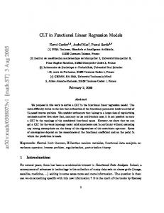
Now we can call function fRegress, which returns various results in a list object that we call fRegressList. fRegressList = fRegress(annualprec,templist,betalist) The command names(fRegressList) reveals a component betaestlist containing the estimated regression coefficient functions. Each of these is a functional parameter object. We can plot the estimate of the regression function for the temperature profiles with the commands betaestlist = fRegressList$betaestlist tempbetafd = betaestlist[[2]]$fd plot(tempbetafd, xlab="Day", ylab="Beta for temperature") Figure 9.1 shows the result. The intercept term can be obtained from coef( betaestlist[[1]]); its value in this case is 0.0095. We will defer commenting on these estimates until we consider the next more sophisticated strategy. We need to assess the quality of this fit. First, let us extract the fitted values defined by this model and compute the residuals. We will also compute error sums of squares associated with the fit as well as for the fit using only a constant or intercept. annualprechat1 = fRegressList$yhatfdobj annualprecres1 = annualprec - annualprechat1 SSE1.1 = sum(annualprecres1ˆ2) SSE0 = sum((annualprec - mean(annualprec))ˆ2)
135
0.0005 0.0000 −0.0010 −0.0005
Beta for temperature
0.0010
0.0015
9.4 Three Estimates of the Regression Coefficient Predicting Annual Precipitation
0
100
200
300
Day
Fig. 9.1 Estimated β (t) for predicting log annual precipitation from average daily temperature using five Fourier basis functions.
We can now compute the squared multiple correlation and the usual F-ratio for comparing these two fits. RSQ1 = (SSE0-SSE1.1)/SSE0 Fratio1 = ((SSE0-SSE1)/5)/(SSE1/29) The squared multiple correlation is 0.80, and the corresponding F-ratio with 5 and 29 degrees of freedom is 22.6, suggesting a fit to the data that is far better than we would expect by chance.
9.4.2 Coefficient β Estimate Using a Roughness Penalty There are two ways to obtain a smooth fit. The simplest is to use a low-dimensional basis for β (t). However, we can get more direct control over what we mean by “smooth” by using a roughness penalty. The combination of a high-dimensional basis with a roughness penalty reduces the possibilities that either (a) important features are missed or (b) extraneous features are forced into the image by using a basis set that is too small for the application. Suppose, for example, that we fit (9.2) by minimizing the penalized sum of squares Z
PENSSEλ (α0 , β ) = ∑[yi − α0 −
Z
xi (t)β (t)dt]2 + λ
[Lβ (t)]2 dt.
(9.4)
136
9 Functional Linear Models for Scalar Responses
This allows us to shrink variation in β as close as we wish to the solution of the differential equation Lβ = 0. Suppose, for example, that we are working with periodic data with a known period. As noted with expression (5.11), the use of a harmonic acceleration operator, Lβ = (ω 2 )Dβ + D3 β , places no penalty on a simple sine wave and increases the penalty on higher-order harmonics in a Fourier approximation approximately in proportion to the sixth power of the order of the harmonic. (In this expression, ω is determined by the period, which is assumed to be known.) Thus, increasing the penalty λ in (9.4) forces β to look more and more like β (t) = c1 + c2 sin(ω t) + c3 cos(ω t). More than one functional covariate can be incorporated into this model and scalar covariates may also be included. Let us suppose that in addition to yi we have measured p scalar covariates zi = (zi1 , . . . , zip ) and q functional covariates xi1 (t), . . . , xiq (t). We can put these into a linear model as follows q
Z
yi = α0 + z0i α + ∑
xi j (t)β j (t)dt + εi ,
(9.5)
j=1
where zi is the p − vector of scalar covariates. A separate smoothing penalty may be employed for each of the β j (t), j = 1, . . . , q. Using (9.5), we can define a least-squares estimate as follows. We define Z by: 0 R R z1 x11 (t)Φ 1 (t)dt · · · x1q (t)Φ q (t) .. Z = ... . . z0n
R
xn1 (t)Φ 1 (t)dt · · ·
R
xnq (t)Φq (t)
Here Φk is the basis expansion used to represent βk (t). We also define a penalty matrix 0 ··· ··· ··· 0 λ1 R1 · · · 0 (9.6) R(λ ) = . . . . . ... .. .. 0
· · · λq Rq
where Rk is the penalty matrix associated with the smoothing penalty for βk and λk is the corresponding smoothing parameter. With these objects, we can define ¢−1 0 ¡ Zy bˆ = Z0 Z + R(λ ) to hold the vector of estimated coefficients αˆ along with the coefficients defining each estimated coefficient function βˆk (t) estimated by penalized least squares. These are then extracted to form the appropriate functional data objects. Now let us apply this approach to predicting the log annual precipitations. First, we set up a harmonic acceleration operator, as we did already in Chapter 5. Lcoef = c(0,(2*pi/365)ˆ2,0)
9.4 Three Estimates of the Regression Coefficient Predicting Annual Precipitation
137
harmaccelLfd = vec2Lfd(Lcoef, c(0,365)) Now we replace our previous choice of basis for defining the β estimate by a functional parameter object that incorporates both this roughness penalty and a level of smoothing: betabasis = create.fourier.basis(c(0, 365), 35) lambda = 10ˆ12.5 betafdPar = fdPar(betabasis, harmaccelLfd, lambda) betalist[[2]] = betafdPar These now allow us to invoke fRegress to return the estimated functional coefficients and predicted values: annPrecTemp
= fRegress(annualprec, templist, betalist) betaestlist2 = annPrecTemp$betaestlist annualprechat2 = annPrecTemp$yhatfdobj The command print(fRegressList$df) indicates the degrees of freedom for this model, including the intercept, is 4.7, somewhat below the value of 6 that we used for the simple model above. Now we compute the usual R2 and F-ratio statistics to assess the improvement in fit achieved by including temperature as a covariate. SSE1.2 = sum((annualprec-annualprechat2)ˆ2) RSQ2 = (SSE0 - SSE1.2)/SSE0 Fratio2 = ((SSE0-SSE1.2)/3.7)/(SSE1/30.3) The squared multiple correlation is now 0.75, a small drop from the value for the simple model, due partly to using fewer degrees of freedom. The F-ratio is 25.1 with 3.7 and 30.3 degrees of freedom, and is even more significant than for the simple model. The reader should note that because a smoothing penalty has been used, the F-distribution only represents an approximation to the null distribution for this model. Figure 9.2 compares predicted and observed values of log annual precipitation. Figure 9.3 plots the coefficient β (t) along with the confidence intervals derived below. Comparing this version with that in Figure 9.1 shows why the roughness penalty approach is to be preferred over the fixed low-dimension strategy; now we see that only the autumn months really matter in defining the relationship, and that the substantial oscillations over other parts of the year in Figure 9.1 are actually extraneous. To complete the picture, we should ask whether we could do just as well with a constant value for β . Here we use the constant basis, run fRegress, and redo the comparison using this fit as a benchmark. The degrees of freedom for this model is now 2. betalist[[2]] = fdPar(conbasis) fRegressList = fRegress(annualprec, templist, betalist) betaestlist = fRegressList$betaestlist
138
9 Functional Linear Models for Scalar Responses
Now we compute the test statics for comparing these models. annualprechat SSE1 RSQ Fratio
= = = =
fRegressList$yhatfdobj sum((annualprec-annualprechat)ˆ2) (SSE0 - SSE1)/SSE0 ((SSE0-SSE1)/1)/(SSE1/33)
2.8 2.6 2.2
2.4
annualprec
3.0
3.2
3.4
We find that R2 = 0.49 and F = 31.3 for 1 and 33 degrees of freedom, so that the contribution of our model is also important relative to this benchmark. That is, functional linear regression is the right choice here.
2.2
2.4
2.6
2.8
3.0
annualprechat
Fig. 9.2 Observed log annual precipitation values plotted against values predicted by functional linear regression on temperature curves using a roughness penalty.
9.4.3 Choosing Smoothing Parameters How did we come up with λ = 1012.5 for the smoothing parameter in this analysis? Although smoothing parameters λ j can certainly be chosen subjectively, we can also consider cross-validation as a way of using the data to define smoothing level. To (−i) (−i) define a cross-validation score, we let αλ and βλ be the estimated regression parameters estimated without the ith observation. The cross-validation score is then ¸2 · Z (−i) (−i) CV(λ ) = ∑ yi − αλ − xi (t)βλ dt . N
i=1
(9.7)
139
5e−04 0e+00 −5e−04
Temperature Reg. Coeff.
1e−03
9.4 Three Estimates of the Regression Coefficient Predicting Annual Precipitation
0
100
200
300
Day
Fig. 9.3 Estimate β (t) for predicting log annual precipitation from average daily temperature with a harmonic acceleration penalty and smoothing parameter set to 1012.5 . The dashed lines indicate pointwise 95% confidence limits for values of β (t).
Observing that
¡ ¢−1 0 yˆ = Z Z0 Z + R(λ ) Z y = Hy
standard calculations give us that N
CV(λ ) = ∑
i=1
µ
yi − yˆi 1 − Hii
¶2 .
(9.8)
We can similarly define a generalized cross-validation score: 2
GCV(λ ) =
∑ni=1 (yi − yˆi ) . (n − Tr(H))2
(9.9)
These quantities are returned by fRegress for scalar responses only. This GCV(λ ) was discussed (in different notation) in Section 5.2.5. For a comparison of CV and GCV including reference to more literature, see Section 21.3.4, p. 368, in Ramsay and Silverman (2005). The following code generates the data plotted in Figure 9.4. loglam = seq(5,15,0.5) nlam = length(loglam) SSE.CV = matrix(0,nlam,1) for (ilam in 1:nlam) { lambda = 10ˆloglam[ilam]
9 Functional Linear Models for Scalar Responses
1.1 1.2 1.3 1.4 1.5 1.6 1.7
Cross−validation score
140
6
8
10
12
14
log smoothing parameter lambda
Fig. 9.4 Cross-validation scores CV(λ ) for fitting log annual precipitation by daily temperature profile, with a penalty on the harmonic acceleration of β (t).
betalisti = betalist betafdPar2 = betalisti[[2]] betafdPar2$lambda = lambda betalisti[[2]] = betafdPar2 fRegi = fRegress.CV(annualprec, templist, betalisti) SSE.CV[ilam] = fRegi$SSE.CV }
9.4.4 Confidence Intervals Once we have conducted a functional linear regression, we want to measure the precision to which we have estimated each of the βˆ j (t). This can be done in the same manner as confidence intervals for probes in smoothing. Under the usual independence assumption, the εi are independently normally distributed around zero with variance σe2 . The covariance of ε is then
Σ = σe2 I. Following a δ -method calculation, the sampling variance of the estimated parameter vector bˆ is
9.4 Three Estimates of the Regression Coefficient Predicting Annual Precipitation
141
¢−1 0 ¡ ¢−1 £ ¤ ¡ Z Σ Z Z0 Z + R . Var bˆ = Z0 Z + R(λ ) Naturally, any more general estimate of Σ , allowing correlation between the errors, can be used here. We can now obtain confidence intervals for each of the β j (t). To do this, we need an estimate of σe2 . This can be obtained from the residuals. The following code does the trick in R: resid = annualprec - annualprechat SigmaE.= sum(residˆ2)/(35-fRegressList$df) SigmaE = SigmaE.*diag(rep(1,35)) y2cMap = tempSmooth$y2cMap stderrList = fRegress.stderr(fRegressList, y2cMap, SigmaE) Here the second argument to fRegress.stderr is a place-holder for a projection matrix that will be used for functional responses (see Chapter 10). We can then plot the coefficient function β (t) along with plus and minus two times its standard error to obtain the approximate confidence bounds in Figure 9.3: betafdPar = betaestlist[[2]] betafd = betafdPar$fd betastderrList = stderrList$betastderrlist betastderrfd = betastderrList[[2]] plot(betafd, xlab="Day", ylab="Temperature Reg. Coeff.", ylim=c(-6e-4,1.2e-03), lwd=2) lines(betafd+2*betastderrfd, lty=2, lwd=1) lines(betafd-2*betastderrfd, lty=2, lwd=1) We note that, like the confidence intervals that we derived for probes, these intervals are given pointwise and do not take account of bias or of the choice of smoothing parameters. In order to provide tests for the overall effectiveness of the regression we resort to permutation tests described in Section 9.5 below.
9.4.5 Scalar Response Models by Functional Principal Components A third alternative for functional linear regression with a scalar response is to regress y on the principal component scores for functional covariate. The use of principal components analysis in multiple linear regression is a standard technique: 1. Perform a principal components analysis on the covariate matrix X and derive the principal components scores fi j for each observation i on each principal component j. 2. Regress the response yi on the principal component scores ci j .
142
9 Functional Linear Models for Scalar Responses
We often observe that we need only the first few principal component scores, thereby considerably improving the stability of the estimate by increasing the degrees of freedom for error. In functional linear regression, we consider the scores resulting from a functional principal components analysis of the temperature curves conducted in Chapter 7. We can write ¯ + ∑ ci j ξ j (t). xi (t) = x(t) j>=0
Regressing on the principal component scores gives us the following model: yi = β0 + ∑ ci j β j + εi .
(9.10)
R
¯ If we substitute this in (9.10), we Now we recall that ci j = ξ j (t)(xi (t) − x(t))dt. can see that Z yi = β0 + ∑ β j ξ j (t)(xi j (t) − x(t))dt ¯ + εi . This gives us
β (t) = ∑ β j ξ j (t).
Thus, (9.10) expresses exactly the same relationship as (9.2) when we absorb the mean function into the intercept:
β˜0 = β0 −
Z
¯ β (t)x(t)dt.
The following code carries out this idea for the annual cycles in daily temperatures at 35 Canadian weather stations. First we resmooth the data using a saturated basis with a roughness penalty. This represents rather more smoothing than in the earlier version of tempfd that did not use a roughness penalty. daybasis365=create.fourier.basis(c(0, 365), 365) lambda =1e6 tempfdPar =fdPar(daybasis365, harmaccelLfd, lambda) tempfd =smooth.basis(day.5, daily$tempav, tempfdPar)$fd Next we perform the principal components analysis, again using a roughness penalty. lambda tempfdPar temppca harmonics
= = = =
1e0 fdPar(daybasis365, harmaccelLfd, lambda) pca.fd(tempfd, 4, tempfdPar) temppca$harmonics
Approximate pointwise standard errors can now be constructed out of the covariance matrix of the β j :
9.5 Statistical Tests
143
var[βˆ (t)] = [ξ1 (t) . . . ξk (t)]Var [β ]
ξ1 (t) .. . . ξk (t)
Since the coefficients are orthogonal, the covariance of the β j is diagonal and can be extracted from the standard errors reported by lm. When smoothed principal components are used, however, this orthogonality no longer holds and the full covariance must be used. The final step is to do the linear model using principal component scores and to construct the corresponding functional data objects for the regression functions. pcamodel = lm(annualprec˜temppca$scores) pcacoefs = summary(pcamodel)$coef betafd = pcacoefs[2,1]*harmonics[1] + pcacoefs[3,1]*harmonics[2] + pcacoefs[4,1]*harmonics[3] coefvar = pcacoefs[,2]ˆ2 betavar = coefvar[2]*harmonics[1]ˆ2 + coefvar[3]*harmonics[2]ˆ2 + coefvar[4]*harmonics[3]ˆ2 The quantities resulting from the code below are plotted in Figure 9.5. In this case the R-squared statistic is similar to the previous analysis at 0.72. plot(betafd, xlab="Day", ylab="Regression Coef.", ylim=c(-6e-4,1.2e-03), lwd=2) lines(betafd+2*sqrt(betavar), lty=2, lwd=1) lines(betafd-2*sqrt(betavar), lty=2, lwd=1) Functional linear regression by functional principal components has been studied extensively. Yao et al. (2005) observes that instead of presmoothing the data, we can estimate the covariance surface directly by a two-dimensional smooth and use this to derive the fPCA. From here the principal component scores can be calculated by fitting the principal component functions to the data by least squares. This can be advantageous when some curves are sparsely observed.
9.5 Statistical Tests So far, our tools have concentrated on exploratory analysis. We have developed approximate pointwise confidence intervals for functional coefficients. However, we have not attempted to formalize these into test statistics. Hypothesis tests provide a formal criterion for judging whether a scientific hypothesis is valid. They also perform the useful function of allowing us to assess “What would the results look like if there really were no relationship in the data?”
9 Functional Linear Models for Scalar Responses
5e−04 0e+00 −5e−04
Temperature Reg. Coeff.
1e−03
144
0
100
200
300
Day
Fig. 9.5 Estimate β (t) for predicting log annual precipitation from average daily temperature using scores from the first three functional principal components of temperature. The dashed lines indicate pointwise 95% confidence limits for values of β (t).
Because of the nature of functional statistics, it is difficult to attempt to derive a theoretical null distribution for any given test statistic since we would need to account for selecting a smoothing parameter as well as the smoothing itself. Instead, the package employs a permutation test methodology. This involves constructing a null distribution from the observed data directly. If there is no relationship between the response and the covariates, it should make no difference if we randomly rearrange the way they are paired. To see what a result might look in this case, we can simply perform the experiment of rearranging the vector of responses while keeping the covariates in the same order and trying to fit the model again. The advantage of this is that we no longer need to rely on distributional assumptions. The disadvantage is that we cannot test for the significance of an individual covariate among many. In order to turn this idea into a formalized statistical procedure, we need a way to determine whether the result we get from the observed data is different from what is obtained by rearranging the response vector. We do this in the classic manner, by deciding on a test statistic that measures the strength of the predictive relationship in our model. We now have a single number which we can compare to the distribution that is obtained when we calculate the same statistic with a randomly permuted response. If the observed test statistic is in the tail of this distribution, we conclude that there is a relationship between the response and covariates. In our case, we compute an F statistic for the regression
9.6 Some Things to Try
145
F=
1 n
Var[ˆy] ∑(yi − yˆi )2
where yˆ is the vector of predicted responses. This statistic varies from the classic F statistic in the manner in which it normalizes the numerator and denominator sums of squares. The statistic is calculated several hundred times using a different random permutation each time. The p value for the test can then be calculated by counting the proportion of permutation F values that are larger than the F statistic for the observed pairing. The following code implements this procedure for the Canadian weather example: F.res = Fperm.fd(annualprec, templist, betalist) Here the observed F statistic (stored in F.res$Fobs) is 3.03, while the 95th quartile of the permutation distribution (F.res$qval) is 0.27, giving strong evidence for the effect.
9.6 Some Things to Try 1. Medfly Data: We reconsider the medfly data described in Section 7.7. a. Perform a functional linear regression to predict the total lifespan of the fly from their egg laying. Choose a smoothing parameter by cross-validation and plot the coefficient function with confidence intervals. b. What is the R2 of your fit to these data? How does this compare with that for the principal components regression you tried earlier? c. Construct confidence intervals for the coefficient function obtained using principal components regression. How do these compare to that for your estimates found using fRegress? Experiment with increasing the smoothing parameter in fRegress and the number of components for principal components regression. d. Conduct a permutation test for the significance of the regression. Calculate the R2 for your regression. 2. Tecator Data: The Tecator data available from http://lib.stat.cmu.edu/datasets/tecator provides an example of functional data in which the domain of the function is not time. Instead, we observe the spectra of meat samples from which we would like to determine a number of chemical components. In particular, the moisture content of the meat is of interest. a. Represent the spectra using a reasonable basis and smoothing penalty.
146
9 Functional Linear Models for Scalar Responses
b. Experiment with functional linear regression using these spectra as covariates for the regression model. Plot the coefficient function along with confidence intervals. What is the R2 for your regression? c. Try using the derivative of the spectrum to predict moisture content. What happens if you use both the derivative and the original spectrum? 3. Diagnostics: Residual diagnostics for functional linear regression is a largely unexplored area. Here are some suggestions for checking regression assumptions for one of the models suggested above. a. Residual by predicted plots can still be constructed, as can QQ plots for residuals. Do these tell you anything about the data? b. In linear regression, we look for curvature in a model by plotting residuals against covariates. In functional linear regression, we would need to plot residuals against the predictor value at each time t. Experiment with doing this at a fine grid of t. Alternatively, you can plot these as lines in three-dimensional space using the lattice or rgl package. c. Do any points concern you as exhibiting undue influence? Consider removing them and measure the effect on your model. One way to get an idea of influence is the integrated squared difference in the βi (t) coefficients. You can calculate this using the inprod function.
9.7 More to Read Functional linear regression for scalar responses has a large associated literature. Models based on functional principal components analysis are found in Cardot et al. (1999), Cardot et al. (2003a) and Yao et al. (2005). Tests for no effect are developed in Cardot et al. (2004), Cardot et al. (2003b) and Delsol et al. (2008). More recent work by James et al. (2009) has focused on using absolute value penalties to insist that β (t) be zero or exactly linear over large regions. Escabias et al. (2004) and James (2002) look at the larger problem of how to adapt the generalized linear model to the presence of a functional predictor variable. M¨uller and Stadtm¨uller (2005) also investigate what they call the generalized functional linear model. James and Hastie (2001) consider linear discriminant analysis where at least one of the independent variables used for prediction is a function and where the curves are irregularly sampled.