Nov 1, 2018 - variance function of observed functional predictors automatically filters .... be potentially applied in many error-contaminated curve time series ...
Functional Linear Regression: Dependence
arXiv:1806.05471v2 [stat.ME] 1 Nov 2018
and Error Contamination Xinghao Qiao1 , Cheng Chen1 , and Shaojun Guo2 1 Department 2 Institute
of Statistics, London School of Economics, U.K.
of Statistics and Big Data, Renmin University of China, P.R. China
Abstract Functional linear regression is an important topic in functional data analysis. Traditionally, one often assumes that samples of the functional predictor are independent realizations of an underlying stochastic process, and are observed over a grid of points contaminated by independent and identically distributed measurement errors. In practice, however, the dynamical dependence across different curves may exist and the parametric assumption on the error covariance structure could be unrealistic. In this paper, we consider functional linear regression with serially dependent functional predictors, when the contamination of predictors by the error is “genuinely functional” with fully nonparametric covariance structure. Inspired by the fact that the autocovariance function of observed functional predictors automatically filters out the impact from the unobservable noise term, we propose a novel autocovariance-based generalized method-of-moments estimate of the slope function. The asymptotic properties of the resulting estimators under different functional scenarios are established. We also demonstrate that our proposed method significantly outperforms possible competitors through intensive simulation studies. Finally, the proposed method is applied to a public financial dataset, revealing some interesting findings. Some key words: Autocovariance; Dependence; Eigenanalysis; Errors-in-predictors; Functional linear regression; Generalized method-of-moments.
1
1
Introduction
In functional data analysis, the linear regression problem depicting the linear relationship between a functional predictor and either a scalar or functional response, has recently received a great deal of attention. See Ramsay and Silverman (2005) for a thorough discussion of the issues involved with fitting such data. For examples of recent research on functional linear models, see Yao et al. (2005); Hall and Horowitz (2007); Crambes et al. (2009); Cho et al. (2013); Chakraborty and Panaretos (2017) and the references therein. We refer to Morris (2015) for an extensive review on recent developments for functional regression. In functional regression literature, one typical assumption is to model functional predictors, denoted by X1 p¨q, . . . , Xn p¨q, as independent realizations of an underlying stochastic process. However, curves can also arise from segments of consecutive measurements over time. Examples include daily curves of financial transaction data (Horvath et al., 2014), intraday electricity load curves (Cho et al., 2013) and daily pollution curves (Aue et al., 2015). Such type of curves, also named as curve time series, violates the independence assumption, in the sense that the dynamical dependence across different curves exists. The other key assumption treats each functional predictor as being either fully observed (Hall and Horowitz, 2007) or incompletely observed, with measurement error, at a grid of time points (Crambes et al., 2009). In the latter case, errors associated with distinct observation points are assumed to be independent and identically distributed, corresponding to a diagonal-constant covariance function for the measurement error process. In the curve time series setting, Xt p¨q are often recorded at discrete points and are subject to dependent and heteroskedastic errors (Bathia et al., 2010). Hence, the resulting error covariance matrix would be “more nonparametric” with varying diagonal entries and nonzero off-diagonal entries. In this paper, we consider the functional linear regression in a time series context, which involves serially dependent functional predictors contaminated by “genuinely functional” errors corresponding to a fully nonparametric covariance structure. We assume that the observed erroneous predictors, which we denote by W1 p¨q, . . . , Wn p¨q, are defined on a compact interval U and are subject to errors in the form of Wt puq “ Xt puq ` et puq,
u P U,
(1)
where the error process tet p¨q, t “ 1, 2, . . .u is a sequence of white noise such that Etet puqu “ 0 for all t and Covtet puq, es pvqu “ 0 for any pu, vq P U 2 provided t ‰ s. We also assume that 2
Xt p¨q and et p¨q are uncorrelated and correspond to unobservable signal and noise components, respectively. This error contamination model was also considered in Bathia et al. (2010). To fit the functional regression model, the conventional least square (LS) approach (Hall and Horowitz, 2007) relies on the sample covariance function of Wt puq, which is not a consistent estimator for the true covariance function of Xt puq, thus failing to account for the contamination that can result in substantial estimation bias. One can possibly implements the LS method in the resulting multiple linear regression after performing dimension reduction for Wt puq to identify the dimensionality of Xt puq (Bathia et al., 2010). However, this approach still suffers from unavoidable uncertainty due to et p¨q, while the inconsistency has been demonstrated by our simulations. Inspired from a simple fact that CovtWt puq, Wt`k pvqu “ CovtXt puq, Xt`k pvqu for any k ‰ 0, which indicates that the impact from the unobservable noise term can be automatically eliminated, we develop an autocovariance-based generalized method-of-moments (AGMM) estimator for the slope function. This procedure makes the good use of the serial dependence information, which is the most relevant in the context of time series modelling. To tackle the problem we consider, the conventional LS approach is not directly applicable in the sense that one cannot separate Xt p¨q from Wt p¨q in equation (1). This difficulty was resolved in Hall and Vial (2006) under the restrictive “low noise” setting, which assumes that the noise et p¨q goes to zero as n grows to infinity. The recent work by Chakraborty and Panaretos (2017) implements the regression calibration approach combined with the low rank matrix completion technique to separate Xt p¨q from Wt p¨q. Their approach relies on the identifiability result that, provided real analytic and banded covariance functions for Xt p¨q and et p¨q, respectively, the corresponding two covariance functions are identifiable (Descary and Panaretos, 2017). However, all the aforementioned methods are developed under the critical independence assumption, which would be inappropriate for the setting that W1 p¨q, . . . , Wn p¨q are serially dependent. The proposed AGMM method has four main advantages. First, it can handle regression with serially dependent observations of the functional predictor. The existence of dynamical dependence across different curves makes our problem tractable and facilitates the development of AGMM. Second, without placing any parametric assumption on the covariance structure of the error process, it relies on the autocovariance function to get rid of the effect from the “genuinely functional” error. Interestingly, it turns out that the operator in
3
AGMM defined based on the autocovariance function of the curve process is identical to the nonnegative operator in Bathia et al. (2010), which is used to assess the dimensionality of Xt p¨q in equation (1). We believe that the autocovariance-based idea adopted in AGMM can be potentially applied in many error-contaminated curve time series modelling problems. Third, the proposed method can be applied to both scalar and functional responses with either finite or infinite dimensional functional predictors. Theoretically we establish relevant convergence rates for our proposed estimators under different model settings. Finally, empirically we illustrate the superiority of AGMM relative to its potential competitors. The rest of the paper is organized as follows. In Section 2, we present the model for regression with dependent functional errors-in-predictors and develop AGMM fitting procedures for both scalar and functional responses. In Section 3, we investigate the asymptotic properties of our proposed estimators for the slope function under different functional scenarios. Section 4 illustrates the finite sample performance of AGMM through a series of simulation studies and a public financial dataset. We summarize our paper and discuss several possible future works in Section 5. We relegate all the technical proofs to the Appendix.
2
Methodology
2.1
Model setup
In this section, we describe the model setup for the functional linear regression with dependent errors-in-predictors we consider. Let L2 pUq denote a Hilbert space of square inteş grable functions defined on U equipped with the inner product xf, gy “ U f puqgpuqdu for f, g P L2 pUq. Given a scalar response Yt , a functional predictor Xt p¨q in L2 pUq, and, without loss of generality, assuming that tYt , Xt p¨qu have been centered to have mean zero, the classical scalar-on-function linear regression model is of the form ż Yt “ Xt puqβ0 puqdu ` εt , t “ 1, . . . , n,
(2)
U
where the errors εt , independent of Xt`k p¨q for any integer k, are generated according to a white noise process and β0 p¨q is the unknown slope function we wish to estimate. We assume that the observed functional predictors W1 p¨q, . . . , Wn p¨q satisfy the error contamination model in equation (1). The existence of the unobservable noise term et p¨q reflects the fact that the curves of interest, Xt p¨q, are not directly observed. Instead, they 4
are recorded on a grid of points and are contaminated by the error process, et p¨q, without assuming any parametric structure on the covariance function of the noise term, denoted by Ce pu, vq “ Covtet puq, et pvqu. This modelling guarantees that all the dynamic elements of Wt p¨q are included in the signal term Xt p¨q and all the white noise elements are absorbed into the noise term et p¨q. Furthermore, we assume that predictor errors et p¨q are uncorrelated with both Xt`k p¨q and εt`k , for all integer k. For an integer k ě 0, we assume that the lag-k autocovariance function of Xt p¨q, denoted by Ck pu, vq “ CovtXt puq, Xt`k pvqu does not depend on t. In particular, C0 pu, vq reduces to the covariance function of Xt p¨q, which admits the Karhunen-Lo´eve expansion, Xt puq “ ş ř8 1 j“1 ξtj φj puq, where ξtj “ U Xt puqφj puqdu and Covpξtj , ξtj 1 q “ λj Ipj “ j q with Ip¨q denoting the indicator function. The eigen-pairs tλj , φj p¨quj“1,2,... satisfy the eigen-decomposition ş C pu, vqφj pvqdv “ λj φj puq with λ1 ě λ2 ě ¨ ¨ ¨ . We say that Xt p¨q is d-dimensional if U 0 λd ‰ 0, and λd`1 “ 0, for some integer d ě 1. When d is finite, β0 p¨q is not identifiable in ş general and here we define β0 p¨q by the minimizer of U β02 puqdu subject to CovtY1 , X1 puqu “ ş řd ´1 C pu, vqβpvqdv, u P U, which implies that β puq “ 0 0 j“1 λj CovpY1 , ξ1j qφj puq. When U d “ 8, all the eigenvalues are nonzero and Xt p¨q is a truly infinite dimensional functional ř ´2 2 object. In this case, provided that 8 j“1 λj tCovpY1 , ξ1j qu ă 8, β0 p¨q can be uniquely exř8 ´1 pressed as β0 puq “ j“1 λj CovpY1 , ξ1j qφj puq. See also Cardot et al. (2003) and He et al. (2010).
2.2
Main idea
In this section, we describe the main idea to facilitate the development of AGMM to estimate β0 p¨q in (2). We choose Xt`k p¨q for k “ 0, 1, . . . , as functional instrumental variables, which are assumed to be uncorrelated with the error εt in (2). Let ż ( X gk pβ, uq “ Cov Yt , Xt`k puq ´ CovtXt pvq, Xt`k puquβpvqdv.
(3)
U
The population moment conditions, Etεt Xt`k puqu “ 0 for any u P U, and equation (2) implies that gkX pβ0 , uq ” 0 for any u P U and k “ 1, . . . .
(4)
In particular, the conventional LS approach is based on (4) with k “ 0. However, this approach is inappropriate when Xt p¨q are replaced by the surrogates Wt p¨q given the fact that CW pu, vq “ CovtWt puq, Wt pvqu “ C0 pu, vq ` Ce pu, vq, and hence the sample version of 5
CW pu, vq is not a consistent estimator for C0 pu, vq. See Hall and Vial (2006) for the discussion on the identifiability of C0 pu, vq and Ce pu, vq under the assumption that the observed curves W1 p¨q, . . . , Wn p¨q are independent and et p¨q decays to zero as n goes to infinity. To separate Xt p¨q from Wt p¨q under the serial dependence scenario, we develop a different approach without requiring the “low noise” condition. Our method is based on the simple fact that CovtYt , Wt`k puqu “ CovtYt , Xt`k puqu and CovtWt puq, Wt`k pvqu “ Ck pu, vq for any k ‰ 0. Then after substituting Xt p¨q by Wt p¨q in (3), we can also represent ż ( gk pβ, uq “ Cov Yt , Wt`k puq ´ CovtWt pvq, Wt`k puquβpvqdv “ gkX pβ, uq, U
and the moment conditions in (4) become gk pβ0 , uq ” 0 for any u P U and k “ 1 . . . , L, where L is some prescribed positive integer. Under the over-identification setting, where the number of moment conditions exceeds the number of parameters, we borrow the idea of generalized methods-of-moments (GMM) based on minimizing the distance from g1 pβ, ¨q, . . . , gL pβ, ¨q to zero. This distance is defined by the quadratic form of Qpβq “
L ÿ L ż ż ÿ k“1 l“1 U
gk pβ, uqΩk,l pu, vqgl pβ, vqdudv,
U
where Ωpu, vq “ tΩk,l pu, vqu1ďk,lďL is an L by L weight matrix whose pk, lq-th element is Ωk,l pu, vq. A suitable choice of Ωpu, vq must satisfy the properties of symmetry and positivedefiniteness (Guhaniyogi et al., 2013), which are, to be specific, (i) Ωkl pu, vq “ Ωlk pv, uq for each k, l “ 1, . . . , L and pu, vq P U 2 ; (ii) for any finite collection of time points u1 , . . . , uT , ` ˘T řT řT T t“1 t1 “1 aput q Ωput , ut1 qaput1 q must be positive for any ap¨q “ a1 p¨q, . . . , aL p¨q . In general, one can choose the optimal weight matrix Ω and implement a two-step GMM. However, this would give a very slight improvement in our simulations. To simplify our derivation and accelerate the computation, we choose the identity weight matrix as Ωk,l pu, vq “ Ipk “ lqIpu “ vq and then minimize the resulting distance of Qpβq “
L ż ÿ k“1 U
6
gk pβ, uq2 du,
over βp¨q P L2 pUq. The minimizer of Qpβq, β0 p¨q, can be achieved by solving BQpβq{Bβ “ 0, i.e. for any u P U, ż !ż L „ż ) ÿ ( Ck pu, zqCov Yt , Wt`k pzq dz ´ Ck pu, zqCk pv, zqdz βpvqdv “ 0. k“1
U
U
(5)
U
To ease our presentation, we define L ż ÿ Rpuq “ Ck pu, zqCovtYt , Wt`k pzqudz
(6)
k“1 U
and Kpu, vq “
L ż ÿ
Ck pu, zqCk pv, zqdz.
(7)
k“1 U
Note that K can be viewed as the kernel of a linear operator acting on L2 pUq, i.e. for any ş f P L2 pUq, K maps f puq to frpuq ” U Kpu, vqf pvqdv. For notational economy, we will use K to denote both the kernel and the operator. Indeed, the nonnegative definite operator K was proposed in Bathia et al. (2010) to identify the dimensionality of Xt p¨q based on Wt p¨q in equation (1). Substituting the relevant terms in (5), β0 p¨q satisfies the following equation ż (8) Rpuq “ Kpu, vqβpvqdv for any u P U, U
which can be understood as a functional extension of the least squares type of population normal equation. Provided that Xt p¨q is d-dimensional, it follows from Proposition 1 of Bathia et al. (2010) that K has exactly d nonzero eigenvalues, θ1 ě θ2 ě ¨ ¨ ¨ ě θd . Let ψ1 , . . . , ψd be the orş thonormal eigenfunctions of K with U Kpu, vqψj pvqdv “ θj ψj puq for j “ 1, . . . , d. Then the ř spectral decomposition of K takes the form of Kpu, vq “ dj“1 θj ψj puqψj pvq. To solve β in (8), one need to take the “inverse” of K. This operator, however, is not generally invertible. To deal with this issue, we use the Moore-Penrose inverse of K, written as K ´1 . Denote the null space of K and its orthogonal complement by kerpKq “ tx P L2 pUq : Kx “ 0u and kerpKqK “ tx P L2 pUq : xx, yy “ 0, @y P kerpKqu, respectively. The ˇ r “ K ˇ kerpKqK , inverse operator K ´1 corresponds to the inverse of the restricted operator K which restricts the domain of K to kerpKqK . See Section 3.5 of Hsing and Eubank (2015) for details. When d ă 8, β0 p¨q is indeed the unique solution of (8) in kerpKqK and can take the form of ż β0 puq “
K
´1
pu, vqRpvqdv “
U
d ÿ j“1
7
θj´1 xψj , Ryψj puq.
(9)
Provided K is a bounded operator under the infinite dimensional setting (d “ 8), K ´1 becomes an unbounded operator, which means it is discontinuous and cannot be estimated in a meaningful way. However, K ´1 is usually associated with another function/operator, the composite function/operator can be reasonably assumed to be bounded, for example the regression operator (Li, 2018). If we further assume that the composite function ş ř ´2 2 K ´1 pu, vqRpvqdv is bounded, or equivalently 8 j“1 θj xψj , Ry ă 8, an unique solution of U (8) exists and is of the form ż β0 puq “
K
´1
pu, vqRpvqdv “
U
2.3
8 ÿ
θj´1 xψj , Ryψj puq.
(10)
j“1
Estimation procedure
In this section, we present the AGMM estimator for β0 p¨q based on the main idea described in Section 2.2. We first provide the sample versions of Ck pu, vq and CovtYt , Wt`k puqu for k “ 1, . . . , L, which are pk pu, vq “ C
n´L n´L 1 ÿ 1 ÿ y Wt puqWt`k pvq and CovtYt , Wt`k puqu “ Yt Wt`k puq. (11) n ´ L t“1 n ´ L t“1
Combing (6), (7) and (11) gives the the natural estimators for Kpu, vq and Rpuq as p vq “ Kpu,
L ż ÿ
pk pu, zqC pk pv, zqdz “ C
k“1 U
L n´L ÿ ÿ ÿ n´L 1 Wt puqWs pvqxWt`k , Ws`k y (12) pn ´ Lq2 k“1 t“1 s“1
and p Rpuq “
L ż ÿ
pk pu, zqCovtY y t , Wt`k pzqudz “ C
k“1 U
L n´L ÿ ÿ n´L ÿ 1 Wt puqYs xWt`k , Ws`k y, pn ´ Lq2 k“1 t“1 s“1 (13)
respectively. Note we choose a fixed integer L ą 1, as K pulls together the information at different lags, while L “ 1 may lead to spurious estimation results. See Section 2.5 for details on the selection of L. p and thus obtain the estimated eigen-pairs tθpj , ψpj p¨qu We next perform an eigenanlysis on K for j “ 1, 2, . . . . When the number of functional observations n is large, the accumulated p are relatively small, thus resulting in smooth errors in (12), (13) and the eigenanalysis on K estimates of ψj p¨q and β0 p¨q. We refer to this implementation of our method as Base AGMM 8
for the remainder of the paper. However, in the setting without a sufficiently large n this version of AGMM suffers from a potential under-smoothing problem that the resulting estimate of β0 p¨q wiggles quite a bit. To overcome this disadvantage, we can impose some level of smoothing in the eigenanalysis through the basis expansion approach, which conp to an approximately equivalent verts the continuous functional eigenanalysis problem for K matrix eigenanalysis task. We explore this basis expansion based AGMM, simply referred to as AGMM from here on. To be specific, let Bpuq be the J-dimensional orthnormal baş sis function, i.e. U BpuqBT puqdu “ IJ , such that for each j “ 1, . . . , J, ψj p¨q can be well approximated by δ Tj Bp¨q, where δ j is the basis coefficients vector. Let ż ż p “ p vqdudv. K BpuqBT pvqKpu, U
U
pj quJ . p leads to the estimated eigen-pairs tpθpj , δ Performing an eigen-decomposision on K j“1 T p Bp¨q. See Then the j-th estimated principal component function is given by ψpj p¨q “ δ j
Section 2.5 for details on the selection of J. A similar basis function expansion technique p θpj , ψpj p¨q, j “ 1, . . . , d, all p can be applied to produce a smooth estimate Rp¨q. Note that K, depend on J, but for simplicity of notation, we will omit the corresponding superscripts where the context is clear. Finally, we substitute the relevant terms in (9) and (10) by their estimated values. We discuss two situations corresponding to d ă 8 and d “ 8 as follows. (i) When Xt p¨q is d-dimensional (d ă 8), we need to select the estimate dp of d in the sense that θp1 , . . . , θpdp are p p and θpp drops dramatically. The estimate βpuq “large” eigenvalues of K of β0 puq is then d`1
given by p βpuq “
dp ÿ
p ψpj puq. θpj´1 xψpj , Ry
(14)
j“1
(ii) When Xt p¨q is an infinite dimensional functional object, we take the standard truncation p to approximate β0 puq in (10). Specifically, approach by using the leading M eigen-pairs of K we obtain the estimated slope function as p βpuq “
M ÿ
p ψpj puq. θpj´1 xψpj , Ry
(15)
j“1
Section 2.5 presents details to select dp and M. However, when d “ 8, the empirical p may be sensitive to the selected value of M. To improve the numerical performance of βp¨q 9
stability, we suggest an alternative ridge-type method to estimate β0 p¨q. Specifically, we propose βpridge puq “
Ă M ÿ
p ψpj puq, pθpj ` ρn q´1 xψpj , Ry
(16)
j“1
Ă is chosen to be reasonably larger than M and ρn is a non-negative ridge parameter. where M See also Hall and Horowitz (2007) for the ridge-type estimator in the classical functional linear regression.
2.4
Generalization to functional response
In this section, we consider the case when the response is also functional. Given a functional response Yt p¨q and a functional predictor Xt p¨q, both of which are in L2 pUq and have mean zero, the function-on-function linear regression takes the form of ż Yt puq “ Xt pvqγ0 pu, vqdv ` εt puq, u P U, t “ 1, . . . , n,
(17)
U
where γ0 pu, vq is the slope function of interest and εt p¨q, independent of Xt`k p¨q for any integer k, are random elements in the underlying separable Hilbert space. We still observe the erroneous version Wt p¨q rather than the signal component Xt p¨q itself, as described in equation (1) and Section 2.1. To estimate the slope function in (17), we develop an AGMM approach analogous to that for the scalar case in Section 2 by solving the normal equation of ż Hpu, vq “ Kpu, wqγpw, vqdw for any v P U,
(18)
U
where Hpu, vq “
řL
ş
k“1 U
Ck pu, zqCovtYt pvq, Wt`k pzqudz with its natural estimator defined
as p vq “ Hpu,
L n´L ÿ ÿ n´L ÿ 1 Wt puqYs pvqxWt`k , Ws`k y. pn ´ Lq2 k“1 t“1 s“1
(19)
p of γ0 under two functional scenarios involving Accordingly, we can provide the estimate γ d ă 8 and d “ 8. (i) Under the finite dimensional setting (d ă 8), γ0 pu, vq is the unique solution of (18) in kerpKqK and can be represented as ż γ0 pu, vq “
K
´1
pu, wqHpw, vqdw “
U
d ÿ j“1
10
θj´1 xψj , Hp¨, vqyψj puq.
(20)
The estimate of γ0 pu, vq is then given by ppu, vq “ γ
dp ÿ
p vqy. θpj´1 ψpj puqxψpj , Hp¨,
(21)
j“1
(ii) Under the infinite dimensional setting (d “ 8), if we assume the boundedness of the ş composite function U K ´1 pu, wqHpw, vqdw in the L2 sense, then the solution of (18) uniquely exists. Approximating the infinite dimensional γ0 pu, vq in (20) by the first M components and substituting the relevant terms by their estimated values, we can obtain the estimated slope function as ppu, vq “ γ
M ÿ
p vqy. θpj´1 ψpj puqxψpj , Hp¨,
(22)
j“1
2.5
Selection of tuning parameters
Implementing AGMM requires choosing L (selected lag length in (5)), M (truncated dimenp when d ă 8) sion in (15) when d “ 8), dp (number of identified nonzero eigenvalues of K and J (dimension of the basis function Bpuq). First, we tend to select a small value of L, as the strongest autocorrelations usually appear at the small time lags and adding more terms p less accurate. Our simulated results suggest that the proposed estimators are will make K not sensitive to the choice of L, therefore we set L “ 5 in our empirical studies. See also Bathia et al. (2010) and Lam et al. (2011) for the relevant discussions. Second, to select M when d “ 8, the typical approach is to find the largest M eigenvalues p such that the corresponding cumulative percentage of variation exceeds the pre-specified of K threshold value, e.g. 90% or 95%. Other available methods to choose M under various situations include the bootstrap test (Bathia et al., 2010) and the eigen-ratio-based estimator (Lam et al., 2011; Lam and Yao, 2012). Third, to determine dp when d ă 8, we take the bootstrap approach proposed in Bathia et al. (2010). Our task is to test the null hypothesis H0 : θd`1 “ 0. We reject H0 if θpd`1 ą cα , where cα is the critical value corresponding to the significant level α P p0, 1q. We summarize the bootstrap procedure as follows. xt p¨q “ řdp ηptj ψpj p¨q, where ηptj “ 1. Define W j“1 xt p¨q. Wt p¨q ´ W
ş U
p Let ept p¨q “ Wt puqψpj puqdu for j “ 1, . . . , d.
xt p¨q ` e˚ p¨q, where e˚ are drawn with 2. Generate a bootstrap sample using Wt˚ p¨q “ W t t replacement from tp e1 , . . . , epn u. 11
p defined in (12), form an estimator K p ˚ by replacing tWt u with 3. In an analogy to K p ˚. tW ˚ u. Then calculate the pd ` 1q-th largest eigenvalue θ˚ of K t
d`1
˚ We repeat Steps 2 and 3 above B-times and reject H0 if the event of tθpd`1 ą θd`1 u occurs more than rp1 ´ αqBs times. Starting with dp “ 1, we sequentially test θd`1 “ 0 and increase p dp by one until the resulting null hypothesis fails to be rejected.
Fourth, to select J, we propose the following G-fold cross validation (CV) approach. 1. Sequentially divide the set t1, . . . , nu into G blockwise groups, D1 , . . . , DG , of approximately equal size. 2. Treat the g-th group as a validation set.
Implement the regularized eigenanalyp p´gq and let ∆ p p´gq “ sis in Section 2.3 on the remaining G ´ 1 groups, compute K ` p´gq ˘ p pp´gq P RJˆd , formed by the top d eigenvectors of K p p´gq . δ ,...,δ 1
d
p pgq based on the validation set. Let θppgq , l “ 1. . . . , d be the p pgq pu, vq and K 3. Compute K l p´gq p´gq T p pgq p p diagonal elements of pδ q K δ . 1
1
We repeat Steps 2 and 3 above G times and choose J as the value that minimize the following mean CV error d G ż ż ! ) ÿ p´gq 2 1 ÿ pgq pp´gq T Tp p pgq pu, vq ´ dudv. δ K θpj pδ q BpuqBpvq CVpJq “ j j G g“1 U U j“1
Given the time break on the training observations, the autocovariance assumption is jeoparp is negligible dized by L “ 5 misutilized lagged terms. However, this effect on the estimate K especially when n is sufficiently large, hence our proposed CV approach can still be applied in practice. See also Bergmeir et al. (2018) for the discussion on various CV methods for time dependent data.
3
Theoretical properties
In this section, we investigate the theoretical properties of our proposed estimators for both scalar-on-function and function-on-function linear regressions. To present the asymptotic results, we need the following regularity conditions.
12
Condition 1 tWt p¨q, t “ 1, 2, . . . u is strictly stationary curve time series. Define the ψmixing with the mixing coefficients ψplq “
sup
|1 ´ P pB|Aq{P pBq|,
l “ 1, 2, . . . ,
0 ,BPF 8 ,P pAqP pBqą0 APF´8 l
where Fij denotes the σ-algebra generated by tWt p¨q, i ď t ď ju. Moreover, it holds that ř8 1{2 plq ă 8. l“1 lψ Condition 2 Ep||Wt ||4 q ă 8 and Epε2t q ă 8. The presentation of the ψ-mixing condition in Condition 1 is mainly for technical convenience. See Section 2.4 of Bosq (2000) on the mixing properties of curve time series. Condition 2 is the standard moment assumption in functional regression literature (Hall and Horowitz, 2007; Chakraborty and Panaretos, 2017). Condition 3 (i) When d is fixed, θ1 ą ¨ ¨ ¨ ą θd ą 0 “ θd`1 ; (ii) When d “ 8, θ1 ą θ2 ą ¨ ¨ ¨ ą 0, and there exist some positive constants c and α ą 1 such that θj ´ θj`1 ě cj ´α´1 for j ě 1; (iii) The eigenfunctions tψj p¨qu8 j“1 are continuous on the compact set U and satisfy supjě1 supuPU |ψj puq| “ Op1q. Condition 4 When d “ 8, β0 puq “
ř8
j“1 bj ψj puq
and there exist some positive constants
τ ě α ` 1{2 and C such that |bj | ď Cj ´τ for j ě 1. Condition 3 restricts the eigen-structure of K and assumes that all the nonzero eigenvalues of K are distinct from each other. When d “ 8, Condition 3 (ii) prevents gaps between adjacent eigenvalues from being too small. The parameter α determines the tightness of eigen-gaps with larger values of α yielding tighter gaps. This condition also indicates that ř ř8 ´α´1 θj ě cα´1 j ´α as θj “ 8 , and can be used to derive the conk“j pθk ´ θk`1 q ě c k“j k vergence rates of estimated eigen-pairs. See also Hall and Horowitz (2007) and Qiao et al. (2018). Under the d “ 8 setting, Condition 4 restricts the true slope function based on the expansion of β0 p¨q using the eigenfunctions of K. The parameter τ determines the decay rate of slope basis coefficients, tbj u8 j“1 . The assumption τ ě α ` 1{2 can be interpreted as requiring that β0 be sufficiently smooth relative to K, the smoothness of which can be implied by θj ě cα´1 j ´α with α ą 1 from Condition 3(ii). See Hall and Horowitz (2007) for an analogous condition in functional linear regression. 13
Before presenting Theorems 1 and 2, which correspond to the asymptotic results for the functional linear regression with scalar and functional responses respectively, we first solidify a some notation. For any univariate function f, define ||f || “ xf, f y. We denote by ||A||S the Hilbert-Schmidt norm for any bivariate function A. The notation an — bn for positive an and bn means that the ratio an {bn is bounded away from zero and infinity. To obtain βp in (14) under the d ă 8 setting, we use the consistent estimator for d defined as dp “ #tj : θpj ě �n u, where �n satisfies the condition in Theorem 1 (i) below. Then by Theorem 3 of Bathia et al. (2010), dp converges in probability to d as n Ñ 8. Theorem 1 Suppose that Conditions 1–4 hold. The following assertions hold as n Ñ 8 : (i) Let �n Ñ 0 and �2n n Ñ 8 as n Ñ 8. When d is fixed, then ` ˘ ||βp ´ β0 || “ OP n´1{2 . (ii) When d “ 8, if we further assume that M — n1{p2α`2τ q , then ` ˘ ` 2τ ´1 ˘ }βp ´ β0 }2 “ OP M 2α`1 n´1 ` M ´2τ `1 “ OP n´ 2α`2τ . We provide remarks on different convergence rates under two functional scenarios. First, when d is fixed, the standard parametric root-n rate is achieved. Second, when d “ 8, the convergence rate is governed by two sets of parameters (1) dimensionality parameter, sample size (n); (2) internal parameters, truncated dimension of the curve time series (M ), decay rate of the lower bounds for eigenvalues (α), decay rate of the upper bounds for slope basis coefficients (τ ). It is easy to see that larger values of α (tighter eigen-gaps) yield a slower convergence rate, while increasing τ enhances the smoothness of β0 p¨q, thus resulting in a faster rate. The convergence rate consists of two terms, which reflects our familiar variance-bias tradeoff as commonly considered in nonparametric statistics. In particular, the bias is bounded by OpM ´τ `1{2 q and the variance is of the order OP pM 2α`1 n´1 q. To balance both terms, we choose the truncated dimension, M — n1{p2α`2τ q , while the optimal convergence rate then becomes OP tn´p2τ ´1q{p2α`2τ q u. It is also worth noting that this rate is slightly slower than the minimax rate OP tn´p2τ ´1q{pα`2τ q u developed in Hall and Horowitz (2007), which considers independent observations of the functional predictor without any error contamination. In fact, we tackle a more difficult functional linear regression problem, where extra complications come from the serial dependence and functional error contamination. From a theoretical perspective, whether the rate in part (ii) is optimal in the minimax sense is still of interest and requires further investigation. 14
Before presenting the asymptotic results for the function-on-function linear regression, we first list two regularity conditions in Conditions 5 and 6 below, which are substitutes of Conditions 2 and 4, respectively, in the functional response case. Condition 5 Ep||Wt ||4 q ă 8 and Ep||εt ||2 q ă 8. Condition 6 When d “ 8, γ0 pu, vq “
ř8 ř8
`“1 bj` ψj puqψ` pvq
j“1
and there exist some positive
constants τ ě α ` 1{2 and C such that |bj` | ď Cpj ` `q´τ ´1{2 for j, ` ě 1. Theorem 2 Suppose that Conditions 1, 3, 5 and 6 hold. The following assertions hold as nÑ8: (i) Let �n Ñ 0 and �2n n Ñ 8 as n Ñ 8. When d is fixed, then γ ´ γ0 ||S “ OP pn´1{2 q. ||p (ii) When d “ 8, if we further assume that M — n1{p2α`2τ q , then ` ˘ ` 2τ ´1 ˘ ||p γ ´ γ0 ||2S “ OP M 2α`1 n´1 ` M ´2τ `1 “ OP n´ 2α`2τ .
4
Empirical studies
4.1
Simulation study
In this section, we evaluate the finite sample performance of AGMM by a number of simulation studies. The observed predictor curves, Wt puq, u P r0, 1s, are generated from equation (1) with Xt puq “
d ÿ
ξtj φj puq and et puq “
j“1
10 ÿ
νtj ζj puq,
j“1
where tξtj uTt“1 follows a linear AR(1) process with the coefficient p´1qj p0.9 ´ 0.5j{dq. The ř slope functions are generated by β0 puq “ dj“1 bj φj puq, where bj ’s take values from the first d components in p2, 1.6, ´1.2, 0.8, ´1, ´0.6q. We generate responses Y1 , . . . , Yn from equation (2), where εt are independent N p0, 1q variables. Finally, we consider two different scenarios to generate tφj p¨qudj“1 , tζj p¨qu10 j“1 and tνtj unˆ10 . Example 1: This example is taken from Bathia et al. (2010) with φj puq “
? 2 cospπjuq, 15
ζj puq “
? 2 sinpπjuq,
and the innovations νtj being independent standard normal variables. We compare two versions of AGMM with three competing methods: covariance-based LS (CLS), covariance-based GMM (CGMM), autocovariance-based LS (ALS). The three competing approaches are implemented as follows. In the first two methods, we perform pW , which converts the functional linear eigenanalysis on the estimated covariance function C regression to the multiple linear regression, and then implement either LS or GMM. The truncated dimension was chosen such that the selected principal components can explain more than 90% of the variation in the trajectory. We also tried the bootstrap method in Hall and Vial (2006) or to set a larger threshold level, e.g. 95%. However neither approach performed well, so we do not report the results here. The third ALS method relies on the p and the subsequent implementation eigenanalysis on the estimated autocovariance-based K of LS. In a similar fashion to the difference between Base AGMM and AGMM, we refer to each of the unregularized method as the “base” version. d=4
d=6
0.0
0.2
0.4
u
0.6
0.8
1.0
0
β(u)
−6
−4
−4
−4
−2
−2
−2
0
β(u)
0
β(u)
2
2
2
4
4
4
6
6
d=2
0.0
0.2
0.4
u
0.6
0.8
1.0
0.0
0.2
0.4
u
0.6
0.8
1.0
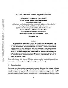
Figure 1: Example 1 with n “ 800 and d “ 2, 4, 6: Comparison of true βp¨q functions (black solid) with median estimates over 100 simulation runs for AGMM (red solid), Base AGMM (red dashed), CLS (cyan solid), Base CLS (cyan dashed), Base CGMM (green dotted) and Base ALS (gray dash-dotted).
The performance of four types of approaches are examined based on the mean integrated ş p p squared error for βpuq, i.e. Er tβpuq ´ β0 puqu2 dus. We consider different settings with d “ 2, 4, 6 and n “ 200, 400, 800, and ran each simulation 100 times. The regularized versions of CGMM and ALS did not give improvements in our simulation studies, so we do not report their results here. Figure 1 provides a graphical illustration of the results for n “ 800 and d “ 2, 4, 6. The black solid lines correspond to the true βpuq from which the data were 16
generated. The median most accurate estimate is also plotted for each of the competing methods. It is easy to see that the AGMM methods apparently provide the highest level of accuracy. The top part of Table 1 reports numerical summaries for all simulation scenarios. We can observe that the advantage of AGMM over Base AGMM is prominent especially when either d or n is relatively small, while AGMM methods are superior to the competing methods when n “ 400 or 800. However, under the setting with n “ 200 and d “ 4 or 6, the bootstrap test in Section 2.5 could not select dp very accurately, thus resulting in AGMM estimates inferior to some competitors. Table 1: Example 1: The mean and standard error (in parentheses) of the mean integrated p squared error for βpuq over 100 simulation runs. The lowest values are in bold font. dp
n
200
Est
400
800
200
True
400
800
d
Base CLS
CLS
Base CGMM
Base ALS
Base AGMM
AGMM
2
1.320(0.026)
1.315(0.025)
2.215(0.099)
1.619(0.044)
1.187(0.052)
0.720(0.033)
4
1.360(0.028)
1.340(0.028)
2.128(0.093)
2.451(0.102)
2.053(0.117)
1.704(0.107)
6
1.337(0.030)
1.320(0.029)
1.912(0.102)
2.150(0.092)
1.847(0.098)
1.612(0.072)
2
1.184(0.018)
1.181(0.019)
1.891(0.090)
1.338(0.026)
0.772(0.034)
0.498(0.028)
4
1.198(0.021)
1.199(0.021)
1.939(0.090)
1.316(0.028)
0.701(0.034)
0.584(0.034)
6
1.159(0.023)
1.154(0.022)
1.519(0.087)
1.323(0.034)
0.824(0.045)
0.745(0.037)
2
1.159(0.012)
1.158(0.012)
1.792(0.080)
1.161(0.013)
0.346(0.013)
0.211(0.012)
4
1.161(0.014)
1.160(0.014)
1.762(0.105)
1.122(0.014)
0.336(0.015)
0.247(0.012)
6
1.123(0.014)
1.122(0.014)
1.297(0.091)
1.119(0.016)
0.348(0.016)
0.350(0.018)
2
1.402(0.032)
1.238(0.030)
0.774(0.044)
1.637(0.044)
1.196(0.052)
0.718(0.033)
4
1.365(0.030)
1.191(0.029)
0.924(0.056)
1.515(0.043)
1.214(0.071)
0.797(0.046)
6
1.345(0.028)
1.272(0.027)
1.150(0.065) 1.465(0.036)
1.378(0.070)
1.196(0.057)
2
1.226(0.019)
1.145(0.019)
0.503(0.027)
1.336(0.026)
0.772(0.034)
0.498(0.028)
4
1.199(0.021)
1.139(0.021)
0.529(0.024)
1.237(0.022)
0.653(0.032)
0.488(0.029)
6
1.166(0.023)
1.139(0.022)
0.656(0.038) 1.170(0.023)
0.726(0.039)
0.704(0.042)
2
1.174(0.012)
1.136(0.012)
0.269(0.011)
1.161(0.013)
0.346(0.013)
0.211(0.012)
4
1.165(0.014)
1.131(0.014)
0.324(0.014)
1.130(0.014)
0.333(0.015)
0.245(0.012)
6
1.121(0.014)
1.119(0.014)
0.323(0.016) 1.106(0.015)
0.336(0.015)
0.334(0.016)
To investigate the performance of AGMM after excluding the negative impact from the low accuracy of dp especially when n “ 200, we also implement an “oracle” version, which uses the true d in the estimation. The numerical results are reported in the bottom part of Table 1. We can observe that GMM methods are superior to their LS versions, while CGMM slightly outperforms AGMM. These observations are due to the facts that, (i) top 17
d eigenvalues for CW and K correspond to the same signal components in Example 1, (ii) GMM methods are capable of removing the impact from the noise term, (iii) the estimate pW in CGMM does not consider the functional error, while K p in AGMM would suffer from C error accumulations. To better demonstrate the superiority of AGMM, we explore Example 2 below, where the covariance-based approach would fail to identify the signal components but its autocovariance-based version could. Example 2: We generate tζj p¨qu10 j“1 from a 10-dimensional orthonormal Fourier basis ? ? function, t 2 cosp2πjuq, 2 sinp2πjuqu5j“1 , and set φj puq “ ζj puq for j “ 1, . . . , d. The innovations νtj are independently sampled from N p0, σj2 q with $ ’ &p1{2qj´1 , for j “ 1, . . . , 6, 2 σj “ ’ %p2.6 ´ 0.1jq ˆ 1.1pd{2´3q , for j “ 7, . . . , 10. In this example, provided the fact that tφj p¨qudj“1 shares the common basis functions with the first d elements in tζj p¨qu10 j“1 , we can calculate the variation in the trajectory explained by each of the 10 components under the population level. See Table 3 of the Supplementary Material for details. Take d “ 4 as an illustrative example, the autocovariance-based methods can correctly identify the 4 signal components, while CLS and CGMM would mis-identify “7” and “8” as the signal components. Table 2 gives numerical summaries under the “oracle” scenario with true d in the estimation. As we would expect, two versions of AGMM provide substantially improved estimates, while Base AGMM is outperformed by AGMM in most of the cases. Under the scenario that dp is selected by the bootstrap approach, Figure 2 and Table 2 provide the graphical and numerical results, respectively. We observe similar trends as in Figure 1 and Table 1 with AGMM methods providing highly significant improvements over all the competitors.
4.2
Real data analysis
In this section, we illustrate the proposed AGMM using a public financial dataset. Let Pt puj q, t “ 1, . . . , n, j “ 1, . . . , T be the price of a financial asset at time uj on the t-th trading day. Denote the cumulative intraday return (CIDR) trajectory, in percentage, by “ ‰ rt puj q “ 100 logtPt puj qu ´ logtPt pu1 qu , where u1 is the opening time of the trading day (Horvath et al., 2014). The dataset we consider was downloaded from https://wrds-web. wharton.upenn.edu/wrds and consists of one-minute resolution prices of Standard & Poor’s 18
d=4
d=6
2
β(u)
−4
−4
−4
−2
−2
−2
0
0
β(u)
0
β(u)
2
4
2
4
6
4
6
d=2
0.0
0.2
0.4
u
0.6
0.8
1.0
0.0
0.2
0.4
u
0.6
0.8
1.0
0.0
0.2
0.4
u
0.6
0.8
1.0
Figure 2: Example 2 with n “ 800 and d “ 2, 4, 6: Comparison of true βp¨q functions (black solid) with median estimates over 100 simulation runs for AGMM (red solid), Base AGMM (red dashed), CLS (cyan solid), Base CLS (cyan dashed), Base CGMM (green dotted) and Base ALS (gray dash-dotted).
100 index and inclusive stocks from n “ 251 trading days in year 2017. The trading period (9:30-16:00) with T “ 390 minutes is rescaled onto U “ r0, 1s. We first obtain the smoothed CIDR curves on the Standard & Poor’s 100 index using the standard kernel method, rrm,t puq “ ř pt pT ht q´1 Tj“1 Kht prm,t puj q ´ uq, where Kh puq is a kernel function with bandwidth h. Let σ be the sample standard deviation of rm,t puj q for j “ 1, . . . , T. We use a Gaussian kernel with the optimal bandwidth p ht “ 1.06p σt T ´1{5 (Silverman, 1999). We extend the classical capital asset pricing model (CAPM) [Chapter 5 of Campbell et al. (1997)] to the functional domain by considering the functional linear regression with functional errors-in-predictors as follows ż rt “ α ` Xt puqβpuqdu ` εt ,
rrm,t puq “ Xt puq ` et puq,
(23)
where Xt p¨q and et p¨q represent the signal and error components in rrm,t p¨q, respectively, and “ ‰ rt “ 100 logtPt puT qu ´ logtPt´1 puT qu is the return for a specific stock on the t-th trading day. Note that the slope parameter in the classical CAPM explains how strongly an asset return depends on the market portfolio. Analogously, βp¨q in functional CAPM in (23) can be understood as the functional sensitivity measure of an asset return to the market CIDR trajectory. Figure 3 plots the estimated βp¨q functions using both CLS and AGMM for three largecap-sector stocks, Amazon (ticker AMZN), General Electronic (ticker GE) and Johnson & 19
Table 2: Example 2: The mean and standard error (in parentheses) of the mean integrated p squared error for βpuq over 100 simulation runs. The lowest values are in bold font. dp
n
400
True
800
1200
400
Est
800
1200
d
Base CLS
CLS
Base CGMM
Base ALS
Base AGMM
AGMM
2
1.591(0.059)
0.990(0.046)
1.118(0.078)
1.165(0.030)
0.599(0.038)
0.262(0.026)
4
2.026(0.066)
1.590(0.070)
2.310(0.112)
0.972(0.033)
0.686(0.041)
0.448(0.034)
6
2.310(0.069)
1.932(0.077)
2.722(0.104)
0.938(0.035)
0.825(0.042)
0.676(0.048)
2
1.377(0.051)
0.940(0.038)
0.884(0.085)
0.994(0.019)
0.337(0.020)
0.138(0.010)
4
1.934(0.051)
1.526(0.054)
2.268(0.105)
0.685(0.016)
0.318(0.016)
0.208(0.013)
6
2.160(0.056)
1.872(0.055)
2.859(0.138)
0.575(0.015) 0.339(0.017)
2
1.294(0.053)
0.980(0.048)
0.750(0.081)
0.900(0.013)
0.203(0.011)
0.080(0.005)
4
1.959(0.053)
1.524(0.058)
2.426(0.121)
0.582(0.009)
0.167(0.008)
0.124(0.006)
6
2.270(0.048)
2.002(0.050)
3.092(0.113)
0.494(0.011) 0.217(0.010)
2
0.817(0.012)
0.818(0.012)
0.980(0.059)
1.141(0.026)
0.575(0.030)
0.248(0.018)
4
1.037(0.043)
0.725(0.036)
1.319(0.070)
1.097(0.038)
0.773(0.042)
0.584(0.038)
6
0.913(0.041)
0.811(0.038)
1.305(0.068)
1.164(0.050)
0.999(0.051)
0.955(0.053)
2
0.795(0.010)
0.795(0.010)
0.899(0.055)
0.989(0.019)
0.333(0.020)
0.138(0.009)
4
1.093(0.033)
0.768(0.035)
1.471(0.065)
0.682(0.016)
0.319(0.016)
0.212(0.013)
6
0.859(0.041)
0.809(0.039)
1.139(0.061)
0.571(0.016) 0.335(0.017)
2
0.779(0.007)
0.780(0.007)
0.747(0.044)
0.898(0.012)
0.205(0.012)
0.079(0.005)
4
1.055(0.026)
0.815(0.032)
1.344(0.052)
0.580(0.009)
0.166(0.008)
0.130(0.007)
6
0.813(0.029)
0.808(0.029)
1.159(0.058)
0.492(0.011) 0.216(0.011)
0.364(0.020)
0.248(0.010)
0.369(0.020)
0.243(0.009)
Johnson (ticker JNJ). To identify the finite dimensionality of rrm,t p¨q, we apply the bootstrap test and the eigen-ratio-based estimator (Lam and Yao, 2012). Both approaches suggest to take dp “ 1. We observe a few apparent patterns in Figure 3. First, the AGMM estimates place more positive weights as u increases. This result seems reasonable given the fact that the daily most recent market price would contain the most information about the stock’s closing price. Second, the CLS estimates first dip in the mid-morning and then start to increase until the end of the trading day. In general, the estimates are insensitive to the choice of bandwidth and the shapes of the estimated βp¨q functions by either CLS or AGMM are quite similar across the three stocks.
20
GE
JNJ
4 2
β(u)
β(u)
−1
−2
0
0
0
1
1
2
β(u)
2
4
3
3
6
8
5
AMZN
0.0
0.2
0.4
u
0.6
0.8
1.0
0.0
0.2
0.4
u
0.6
0.8
1.0
0.0
0.2
0.4
u
0.6
0.8
1.0
Figure 3: Estimated βp¨q curves for AGMM (red) and CLS (black) using ht “ pht (solid lines), 0.5p ht (dotted lines) and 2p ht (dashed lines).
5
Discussion
We conclude our paper with several remarks. First, in comparison with the classical functional linear regression, we study a more difficult problem in a time series context by relaxing the critical independence assumption and allowing functional predictors to be corrupted by “genuinely functional” errors. Second, to address the problem we consider, one can possibly adopt the dimension reduction approach for curve time series (Bathia et al., 2010), which transfers the functional linear regression to the multiple linear regression, however the extra uncertainty from the error contamination would still prevent us from using the LS approach while the deficiency of ALS are demonstrated by the simulation studies. Instead, AGMM can successfully solve this issue by using the autocovariance to remove the part due to the noise term. Moreover, the AGMM approach is closely connected to the work of Bathia et al. (2010). In particular, the operator K proposed under our GMM framework is exactly the same as the nonnegative operator in Bathia et al. (2010) based on the same error contamination model in equation (1). We identify several potential directions for future research. First, we can consider extending the current regression model to the multivariate or even high dimensional setting involving p possibly functional erroneous predictors, where p can be very large. Under the independence and large p, small n, setting, some concentration inequalities based on the covariance structure are established in Qiao et al. (2018). It is of great interest to develop the relevant concentration bounds for high dimensional curve time series under our proposed
21
autocovariance-based framework, which would provide a powerful tool to derive the nonasymptotic upper bounds. The second potential extension concerns the functional singular component analysis (FSCA) (Yang et al., 2011) to model a pair of erroneous curve time series. One possible way to tackle this type of bivariate data is to perform FSCA on some autocovairance-based operator, where the impact from the error term can be eliminated. It is worth noting that some functional relationships such as function-on-function regression might also be represented under a FSCA framework, see Cho et al. (2013) for details. Then an analogous autocovariance-based GMM approach could possibly be applied. Third, the convergence rate in Theorem 1(ii) is slightly slower than the one in Hall and Horowitz (2007). It is of great interest to either prove the optimality of our rate or develop the optimal minimax rate under the setting we consider. These topics are beyond the focus of this paper and will be pursued elsewhere.
A
Appendix
Appendices A.1 and A.2 contain all the technical proofs.
A.1
Proof of Theorem 1
Lemma 1 Suppose that Conditions 1–3 hold and xψpj , ψj y ě 0. Then as n Ñ 8, the following results hold: p ´ K||S “ OP pn´1{2 q and supjě1 |θpj ´ θj | “ OP pn´1{2 q. (i) ||K (ii) When d is fixed, ||ψpj ´ ψj || “ OP pn´1{2 q for j “ 1, . . . , d. (iii)When d “ 8, ||ψpj ´ ψj || “ OP pj 1`α n´1{2 q for j “ 1, 2, . . . . Proof. The first result in part (i) can be found in Theorem 1 of Bathia et al. (2010) and p ´ K||S “ hence the proof is omitted. By (4.43) of Bosq (2000), we have sup |θpj ´ θj | ď ||K jě1
´1{2
OP pn
q, which completes the proof for the second result in part (i). To prove parts (ii) ? ? and (iii), let δj “ 2 2 maxtpθj´1 ´ θj q´1 , pθj ´ θj`1 q´1 u if j ě 2 and δ1 “ 2 2pθ1 ´ θ2 q´1 . It p ´ K||S “ OP pδj n´1{2 q. Under follows from Lemma 4.3 of Bosq (2000) that ||ψpj ´ ψj || ď δj ||K Condition 3(i) with a fixed d, root-n rate can be achieved. When d “ 8, Condition 3(ii) and (iii) imply that δj ď Cj α`1 with some positive constant C. This completes our proof for part (iii).
22
p ´ R|| “ OP pn´1{2 q. Lemma 2 Suppose that Conditions 1-2 hold, then ||R Proof. Provided L is fixed, we may set n ” n ´ L. Let S denotes the space consisting of all the operators with a finite Hilbert-Schmidt norm and H denotes the space consisting of all the functions with a finite L2 norm. Let Ztk “ Wt b Wt`k P S and ztk “ Yt Wt`k P H. Now consider the kernel ρ : S ˆ H Ñ H given by ρpA, xq “ Ax˚ with A P S and x P H. ř řn pk p Let ck p¨q “ CovtYt , Wt`k p¨qu. We can represent C c˚ “ n´2 n ρpZtk , zt1 k q, which is 1 k
t“1
t “1
simply a H valued Von Mises’ functional (Borovskikh, 1996). For d ě 1, neither of Ck and pk p ck is zero, it follows from Lemma 3 of Bathia et al. (2010) that E||C c˚ ´ Ck c˚ ||2 “ Opn´1 q. k
k
Then by the Chebyshev inequality, we have p ´ R|| ď ||R
L ÿ
pk p ||C c˚k ´ Ck c˚k || “ OP pn´1{2 q,
k“1
which completes the proof. Lemma 3 Suppose that Condition 2 holds, then ||R|| “ Op1q. ř Proof. By the definitions of Ck and (6), we have ||R|| ď Lk“1 ||Ck ||S ||CovpYt , Wt`k q|| “ řL k“1 ||EtWt puqWt`k pvqu||S ||EpYt Wt`k puqq||. It follows from Cauchy-Schwartz inequality, Condition 2, Fubini Theorem and Jensen’s inequality that ||EtWt puqWt`k pvqu||2S ż ż “ rEtWt puqWt`k pvqus2 dudv ż żU U ”ż ı2 !ż )2 2 2 2 EtWt puq udu ď E Wt puq2 du ă 8. EtWt puq udu EtWt`k pvq udv “ ď U
U
U 2
Similarly, ||EtYt Wt`k puqu|| ď
ş
EpYt2 q U
U 2
EtWt`k puq udu ă 8. Combining the above results
leads to ||R|| “ Op1q. A.1.1
Proof of Theorem 1 (i)
First we provide Lemma 4 to show the consistency of dp to d when d ă 8. Lemma 4 Suppose the Conditions 1, 2, 3 (i) and (iii) hold. Let �n Ñ 0, �2n n Ñ 8 and as ` ˘ n Ñ 8. Then when d ă 8, P dp ‰ d “ Otp�2 nq´1 u Ñ 0. n
Proof. This lemma, which holds for d ă 8, can be found in Theorem 3 of Bathia et al. (2010) and hence the proof is omitted. q vq “ řd θpj ψpj puqψpj pvq and K ´1 pu, vq “ řd θ´1 ψj puqψj pvq. We have the Define Kpu, j“1 j“1 j following result. 23
Lemma 5 Suppose that Conditions 1, 2, 3(i) and (iii) hold. Then the following results hold. q ´1 ´ K ´1 ||S “ OP pn´1{2 q. (i) ||K (ii) ||K ´1 ||S “ Op1q. Proof. Observe that q ´1 ´ K ´1 “ K
d ÿ
pθpj´1 ´ θj´1 qψpj puqψpj pvq `
j“1
d ÿ
θj´1 tψpj puqψpj pvq ´ ψj puqψj pvqu.
j“1
Then by the orthonormality of tψj p¨qu and tψpj p¨qu, we have q ´1 ´ K ´1 ||S ď ||K
d ÿ
θpj´1 θj´1 |θpj ´ θj | ` 2
j“1
d ÿ
θj´1 ||ψpj ´ ψj ||.
(24)
j“1
When d is fixed, the smallest eigenvalue θd is bounded away from zero. It follows from q ´1 ´ Lemma 1 (i),(ii) and (24) that there exists some positive constant C such that ||K K ´1 ||S ď Cpθd´2 ` θd´1 qn´1{2 , which completes the proof for part (i). ř ř Note that ||K ´1 ||S “ || dj“1 θj´1 ψj puqψj pvq||S “ p dj“1 θj´2 q1{2 ď d1{2 θd´1 . Then part (ii) follows as d is fixed and θd is bounded below from zero. Now we organize our proof for part (i) of Theorem 1, i.e. the case when d ă 8. Let ş r q ´1 pu, vqRpvqdv. p βpuq “ UK For a large δ ą 0, by Lemma 4, we have ` ˘ ` ˘ ` ˘ P n1{2 ||βp ´ β0 || ą δ “ P n1{2 ||βp ´ β0 || ą δ, dp “ d ` P n1{2 ||βp ´ β0 || ą δ, dp ‰ d ` ˘ ` ˘ ď P n1{2 ||βr ´ β0 || ą δ, dp “ d ` P dp ‰ d ` ˘ ď P n1{2 ||βr ´ β0 || ą δ ` op1q, which means that, to prove n1{2 ||βp ´ β0 || “ OP p1q, it suffices to show that ||βr ´ β0 || “ OP pn´1{2 q. It is easy to show that q ´1 ´ K ´1 ||S ||R|| p ` ||K ´1 ||S ||R p ´ R||. ||βr ´ β0 || ď ||K
(25)
Then it follows from Lemmas 2, 3 and 5 that ||βr ´ β0 || “ OP pn´1{2 q. This completes our proof for part (i) of Theorem 1. A.1.2
Proof of Theorem 1 (ii)
Without any ambiguity, write xq, Ky, xK, qy and xp, xK, qyy for ż ż ż ż Kpu, vqqpuqdu, Kpu, vqqpvqdv and Kpu, vqppuqqpvqdudv, U
U
U
U
respectively. In Lemma 6, we give expressions for θpj ´ θj and ψpj ´ ψj for j ě 1. 24
Lemma 6 If inf k‰j |θpj ´ θk | ą 0, then ÿ p ´ K, ψk yy ` ψj xψpj ´ ψj , ψj y. ψpj ´ ψj “ pθpj ´ θk q´1 ψk xψˆj , xK
(26)
k:k‰j
Proof. This lemma can be derived from Lemma 5.1 of Hall and Horowitz (2007) and hence the proof is omitted. Now we are ready to prove Theorem 1(ii) under the d “ 8 setting. Let βM puq “ řM ´1 j“1 θj xψj , Ryψj puq. By the triangle inequality, we have ||βp ´ β0 ||2 ď ||βp ´ βM ||2 ` ||βM ´ β0 ||2 . By (10) and orthonormality of tψj p¨qu, we have ||βM ´ β0 ||2 “
(27)
ř8
´2 2 j“M `1 θj xψj , Ry .
It follows
from Condition 4 and some specific calculations that 8 ÿ
||βM ´ β0 ||2 “
8 ÿ
b2j ď C
j“M `1
j ´2τ “ OpM ´2τ `1 q.
(28)
j“M `1
Next we will show the convergence rate of }βp ´ βM }2 . Observe that p ´ βM puq “ βpuq
M ÿ `
M ÿ ˘ ` ˘ p ´ xψj , Ry ψpj puq θpj´1 ´ θj´1 xψj , Ryψpj puq ` θpj´1 xψpj , Ry
j“1
j“1 M ÿ
`
( θj´1 xψj , Ry ψpj puq ´ ψj puq .
j“1
Then we have }βp ´ βM }2 ď 3
M ÿ `
M ÿ ˘ ` ˘ ´1 ´1 2 2 p p ´ xψj , Ry 2 θj ´ θj xψj , Ry ` 3 θpj´2 xψpj , Ry
j“1
j“1 M ÿ
`3M
› ›2 θj´2 xψj , Ry2 ›ψpj ´ ψj ›
j“1
“ 3In1 ` 3In2 ` 3In3 .
(29)
p “ }K p ´K}S and ΩM “ t2∆ p ď δM u. On the event ΩM , we can see that supjďM |θpj ´ Let ∆ θj | ď θM {2, which implies that 2´1 θj ď θpj ď 2θj . Moreover, we can show that P pΩM q Ñ 1 since n1{2 δM Ñ 8 as n Ñ 8. Hence it suffices to work with bounds that are established under the event ΩM . Provided that event ΩM holds, it follows from supjě1 |θpj ´ θj | “ OP pn´1{2 q in Lemma 1(i) and some calculations that M M M ´ ¯ ÿ ÿ ÿ ` ˘2 ´4 ` ˘2 2 ´2 2 p ´1 p In1 ď 4 θj ´ θj θj xψj , Ry “ 4 θj bj θj ´ θj “ OP n θj´2 b2j . j“1
j“1
25
j“1
By Conditions 3–4, we have In1 “ OP pn´1 q ¨
M ´ÿ
¯ ` ˘ ` ˘ j 2α´2τ “ OP pn´1 q ¨ M ` M 2α´2τ `1 “ oP n´1 M 2α`1 .
(30)
j“1
˘ ` Consider the term In3 . By }ψpj ´ ψj } “ OP j 1`α n´1{2 in Lemma 1(iii) and Condition 4, we obtain that In3 ď M
M ÿ
›
b2j ›ψpj
´ ›2 ` ´1 2´2τ `2α`2 ˘ ˘ › ´ ψj “ OP n M “ OP n´1 M 2α`1 ,
(31)
j“1
where the last equality comes from α ą 1 and 2α ´ 2τ ` 4 ď 2α ` 1 implied by Condition 4. Consider the term In2 . On the event ΩM , we have that In2 ď 4
M ÿ
` ˘ p ´ xψj , Ry 2 θj´2 xψpj , Ry
j“1
ď 12
M ÿ
´ ¯ p ´ Ry2 ` xψpj ´ ψj , R p ´ Ry2 θj´2 xψpj ´ ψj , Ry2 ` xψj , R
j“1
ď 12
M ÿ
´ ¯ p ´ R}2 ` }ψpj ´ ψj }2 }R p ´ R}2 , θj´2 xψpj ´ ψj , Ry2 ` }R
(32)
j“1
where the last inequality comes from orthonormality of tψj p¨qu and Cauchy-Schwarz inequality. By Lemma 6 and some calculations, we can represent the term xψpj ´ ψj , Ry as xψpj ´ ψj , Ry “ Rj1 ` Rj2 , where Rj1 “
ř k:k‰j
p ´ K, ψk yy and Rj2 “ θj bj xψpj ´ ψj , ψj y. It follows θk bk pθpj ´ θk q´1 xψpj , xK
from Condition 3–4, Lemma 1 and Cauchy-Schwarz inequality that M ÿ
2 θj´2 Rj2
´1
“ OP pn q ¨
M ´ÿ
j“1
¯ ˘ ` j ´2τ `2α`2 “ oP n´1 M 2α`1 .
(33)
j“1
Note that on the event ΩM , |θpj ´ θj | ď 2´1 |θj ´ θk | for j “ 1, . . . , k ´ 1, k ` 1, . . . , M and hence |θpj ´ θk | ě 2´1 |θj ´ θk |. If we can show that suppθj2 j 2α q´1 jě1
ÿ
θk2 b2k pθj ´ θk q´2 “ Op1q,
(34)
k:k‰j
then, by Condition 4, Lemma 1 and on the event ΩM , we have M ÿ j“1
2 θj´2 Rj1
ď 4
M ÿ
θj´2
j“1
ÿ
p ´ K}2 θk2 b2k pθj ´ θk q´2 }K S
k:k‰j ´1
“ OP pn q ¨
M ÿ
θj´2 θj2 j 2α “ OP pn´1 M 2α`1 q.
j“1
26
(35)
We turn to prove (34) as follows. Denote rj{2s by the largest integer less than j{2. Then ¨ ˛ rj{2s k“2j`1 8 ÿ ÿ ÿ ÿ ‚θk2 b2k pθj ´ θk q´2 . ` θk2 b2k pθj ´ θk q´2 “ ˝ ` k:k‰j
k“2pj`1q
k“rj{2s`1,k‰j
k“1
Observe that for k ě 2pj ` 1q, θj ´ θk “
k´1 ÿ
ż 2pj`1q
pθs ´ θs`1 q ě c j`1
s“j
ˇ2pj`1q c c ´α ´α ˇ s´α´1 ds “ ´ s´α ˇ ě 2 j , α 2α j`1
and for rj{2s ` 2 ď k ď 2j ` 1 but k ‰ j, |θj ´ θk | ě maxpθj ´ θj`1 , θj´1 ´ θj q ě cj ´α´1 . Therefore, 8 ÿ
pθj2 j 2α q´1
θk2 b2k pθj ´ θk q´2 “ Op1q ¨ j 2α´2τ
k“2pj`1q 2j`1 ÿ
pθj2 j 2α q´1
θk2 b2k pθj ´ θk q´2 ď pθj2 j 2α q´1
2j`1 ÿ
( 2 θj2 ` pθj ´ θk q2 b2k pθj ´ θk q´2
k“rj{2s`1
“ Op1q ¨ rj{2s ÿ
θk2 “ Op1q,
k“2pj`1q
k“rj{2s`1
pθj2 j 2α q´1
8 ÿ
θk2 b2k pθj
´ θk q
´2
ď Op1q
k“1
θj´2 j ´2α p1
rj{2s ÿ
` θj2 j 2α`3´2τ q “ Op1q,
θk2 b2k pθk ´ θ2k q´2 “ Op1q ¨ θ12 j 2α´2τ `1 “ Op1q,
k“1
uniformly in j. Then (34) follows. Moreover, it follows from Condition 3, Lemmas 1–3 that M ÿ
p θj´2 }R
2
´1
´ R} “ OP pn M
j“1
2α`1
q and
M ÿ
p ´ R}2 “ OP pn´2 M 4α`3 q. (36) θj´2 }ψpj ´ ψj }2 }R
j“1
Combing the results in (32)–(33) and (35)–(36), we have ´ ¯ In2 “ OP n´2 M 4α`3 ` n´1 M 2α`1 .
(37)
Combining the results in (27),(28) and (37) and choosing M — n1{p2α`2τ q , we obtain that ` ˘ ` 2τ ´1 ˘ }βp ´ β0 }2 “ OP n´2 M 4α`3 ` n´1 M 2α`1 ` M ´2τ `1 “ OP n´ 2α`2τ , which completes the proof.
27
A.2
Proof of Theorem 2
Following the similar arguments used in the proofs for Lemmas 2 and 3 under some regularity conditions, we can show that p ´ H}S “ OP pn´1{2 q and }H}S “ Op1q. }H rpu, vq “ Consider the case when d is fixed. Let γ
ş U
(38)
q ´1 pu, wqHpw, p K vqdw. Then we have
q ´1 ´ K ´1 ||S ||H|| p S ` ||K ´1 ||S ||H p ´ H||S . ||r γ ´ γ0 ||S ď ||K
(39)
It follows from Lemma 5 and (38) that ||r γ ´ γ||S “ OP pn´1{2 ` n´1{2 q “ OP pn´1{2 q. Finally, applying the similar technique used in the proof for part (i) of Theorem 1, we can prove the result in part (i) of Theorem 2. When d “ 8, let γM pu, vq “
řM
´1 j“1 θj ψj puqxψj , Hp¨, vqy.
By the triangle inequality, we
have ||p γ ´ γ0 ||2S ď ||p γ ´ γM ||2S ` ||γM ´ γ0 ||2S .
(40)
It follows from Condition 6 and some specific calculations that }γM ´
γ0 }2S
8 8 ÿ ÿ
“ }
bj` ψj puqψ` pvq}2S
j“M `1 `“1 8 8 ÿ ÿ
b2j`
“
ďC
j“M `1 `“1
8 8 ÿ ÿ
pj ` `q´2τ ´1 “ OpM ´2τ `1 q.
j“M `1 `“1
γ ´ γM ||2S . Observe that It remains to show that the convergence rate of ||p ppu, vq ´ γM pu, vq “ γ
M ÿ `
˘ θpj´1 ´ θj´1 xψj , Hypvqψpj puq
j“1 M ÿ
`
` ˘ p θpj´1 xψpj , Hypvq ´ xψj , Hy pvqψpj puq
j“1 M ÿ
`
( θj´1 xψj , Hypvq ψpj puq ´ ψj puq .
j“1
Then we have, }p γ´
γM }2S
ď 3
M ÿ `
M ÿ › › ˘ ´1 ´1 2 2 p p ´ xψj , Hy›2 θj ´ θj }xψj , Hy} ` 3 θpj´2 ›xψpj , Hy
j“1
` 3M
j“1 M ÿ
› ›2 › ›2 θj´2 ›xψj , Hy› ›ψpj ´ ψj › .
j“1
28
(41)
Following the similar arguments used in the proof for Theorem 1 (ii), we can show that ||p γ ´ γM ||2S “ OP pM 4α`3 n´2 ` M 2α`1 n´1 q.
(42)
Combing the results in (40)–(42) and choosing M — n1{p2α`2τ q , we have ` ˘ ` 2τ ´1 ˘ ||p γ ´ γ0 ||2S “ OP M 2α`1 n´1 ` M ´2τ `1 “ OP n´ 2α`2τ . which completes our proof for part (ii) of Theorem 2.
References Aue, A., Norinho, D. and Hormann, S. (2015). On the prediction of stationary functional time series, Journal of the American Statistical Association 110: 378–392. Bathia, N., Yao, Q. and Ziegelmann, F. (2010). Identifying the finite dimensionality of curve time series, The Annals of Statistics 38: 3352–3386. Bergmeir, C., Hyndman, R. and Koo, B. (2018). A note on the validity of cross-validation for evaluating autoregressive time series prediction, Computational Statistics and Data Analysis 120: 70–83. Borovskikh, Y. V. (1996). U Statistics in Banach Spaces, VSP, Netherlands. Bosq, D. (2000). Linear Processes in Function Spaces - Theory and Applications, Springer, New York. Campbell, J., Lo, A. W. and A.C., M. (1997). The Econometrics of Financial Markets, Princeton University Press, New Jersey. Cardot, H., Ferraty, F. and Sarda, P. (2003). Splines estimators for the functional linear model, Statistica Sinica 13: 571–591. Chakraborty, A. and Panaretos, V. (2017). Regression with genuinely functional errors-incovariates, arXiv:1712.04290. . Cho, H., Goude, Y., Brossat, X. and Yao, Q. (2013). Modeling and forecasting daily electricity load curves: a hybrid approach, Journal of the American Statistical Association 108: 7–21. Crambes, C., Kneip, A. and Sarda, P. (2009). Smoothing splines estimators for functional linear regression, The Annals of Statistics 37: 35–72. Descary, M.-H. and Panaretos, V. (2017). Functional data analysis by matrix completion, To appear in the Annals of Statistics . 29
Guhaniyogi, R., Finley, A. O., Banerjee, S. and Kobe, R. (2013). Modeling complex spatial dependencies: low rank spatially varying cross-covariances with application to soil nutrient data, Journal of Agricultural, Biological and Environmental Statistics 18: 274–298. Hall, P. and Horowitz, J. Z. (2007). Methodology and convergence rates for functional linear regression, The Annals of Statistics 34: 70–91. Hall, P. and Vial, C. (2006). Assessing the finite dimensionality of functional data, Journal of the Royal Statistical Society: Series B 68: 689–705. He, G., Mueller, H. G., Wang, J. L. and Yang, W. (2010). Functional linear regression via canonical analysis, Bernoulli 16: 705729. Horvath, L., Kokoszka, P. and Rice, G. (2014). Testing stationary of functional time series, Journal of Econometrics 179: 66–82. Hsing, T. and Eubank, R. (2015). Theoretical Foundations of Functional Data Analysis, with an Introduction to Linear Operators, John Wiley & Sons, Chichester. Lam, C. and Yao, Q. (2012). Factor modeling for high-dimensional time series: inference for the number of factors, The Annals of Statistics 40: 694–726. Lam, C., Yao, Q. and Bathia, N. (2011). Estimation of latent factors for high-dimensional time series, Biometrika 98: 901–918. Li, B. (2018). Linear operator-based statistical analysis: A useful paradigm for big data, The Canadian Journal of Statistics 46: 79–103. Morris, J. S. (2015). Functional regression, Annual Review of Statistics and Its Application 2: 321–359. Qiao, X., Guo, S. and James, G. (2018). Functional graphical models, Journal of the American Statistical Association in press. Ramsay, J. and Silverman, B. (2005). Functional data analysis (2nd ed.), Springer, New York. Silverman, B. (1999). Density estimation for Statistics and Data Analysis (2nd ed.), Chapman and Hall, London. Yang, W., Mueller, H. G. and Stadtmueller, U. (2011). Functional singular component analysis, Journal of the Royal Statistical Society: Series B 73: 303–324. Yao, F., Mueller, H. G. and Wang, J. L. (2005). Functional linear regression analysis for longitudinal data, The Annals of Statistics 33: 2873–2903.
30
Supplementary Material to “Functional Linear Regression: Dependence and Error Contamination” Xinghao Qiao, Cheng Chen, and Shaojun Guo
This supplementary material contains additional simulation results supporting Section 4.
B
Additional simulation results
For Example 2, Table 3 reports the variance explained by each of the 10 components under the population level. For each of the three parts corresponding to d “ 2, 4 and 6, the second and third rows provide the variance explained by each of the d signal components and 10 error components, respectively. The first row ranks the components based on the overall variance explained by each individual component, where the fourth row displays the corresponding values. Take d “ 4 as an illustrative example, the autocovariance-based approach can correctly identify the first four signal components, while the covariance-based approach can only correctly identify “1” and “2”, but incorrectly select “7” and “8” as signal components. Moreover, we consider another scenario for Example 2 by generating innovations tνtj u from a standard normal distribution, where the variance decomposition is illustrated via Table 4. Under this setting, we can observe that both approaches are capable of correctly identifying the d signal components.
1
Table 3:
The variance explained by each of the components in Example 2. Top d components
identified by covaraicne-based and autocovariance-based approaches are underlined and in bold font, respectively.
Component
d=2
d=4
d=6
1
2
7
8
9
10
3
4
5
6
Signal
1.73 1.19
Error
1.00
0.50
1.57
1.49
1.40
1.32
0.25
0.13
0.06
0.03
Sum
2.73
1.69
1.57
1.49
1.40
1.32
0.25
0.13
0.06
0.03
Component
1
2
7
8
9
10
3
4
5
6
1.38
1.19
Signal
2.50 1.73
Error
1.00
0.50
1.73
1.64
1.55
1.45
0.25
0.13
0.06
0.03
Sum
3.50
2.23
1.73
1.64 1.55
1.45
0.25
0.13
0.06
0.03
Component
1
2
3
9
10
4
5
6
1.47
1.30
1.19
7
8
Signal
3.00 2.16
1.73
Error
1.00
0.50
0.25
1.90
1.70
1.60
0.13
0.06
0.03
Sum
4.00
2.66
1.98
1.90 1.80 1.70
1.60
1.60
1.37
1.22
2
1.80
Table 4: The variance explained by each of the components in Example 2 with tνtj u being N p0, 1q variables. Top d components identified by covaraicne-based and autocovariance-based approaches are underlined and in bold font, respectively.
Component
1
2
3
4
5
6
Signal
1.73
1.19
Error
1.00
Sum
7
8
9
10
1.00
1.00
1.00
1.00
1.00
1.00 1.00 1.00
1.00
2.73
2.19
1.00
1.00
1.00
1.00
1.00 1.00 1.00
1.00
Component
1
2
3
4
5
6
Signal
2.50
1.73
1.38 1.19
Error
1.00
1.00
1.00
1.00
1.00
1.00
1.00 1.00 1.00
Sum
3.50
2.73
2.38
2.19
1.00
1.00
1.00 1.00 1.00 1.00
Component
1
2
3
4
5
6
Signal
3.00
2.16
1.73 1.47
1.30
1.19
Error
1.00
1.00
1.00
1.00
1.00
1.00
1.00 1.00 1.00
1.00
Sum
4.00
3.16
2.73
2.47
2.30
2.19
1.00
1.00
d=2 7
8
9
10
1.00
d=4 7
8
9
10
d=6
3
1.00 1.00