Good models (contd.) â« ... The best linear model minimizes the sum of squared errors ... SS0 has just one degree of fr
Based on material provided by Loughborough University Mathematics Learning Support Centre and. Coventry University Mathematics Support Centre.
relationship between the two variables. Simple linear regression model is then
formulated and the key theoretical results are given without mathematical deriva-.
MS Statistics I. SIMPLE LINEAR REGRESSION. 6.1 THE MODEL. The Simple Linear Regression Model for n observations can be written as yi = β0 + β1xi + εi,.
can get Minitab to list the residuals. The simple linear regression model page 12.
This section shows the very important linear regression model. It's very.
Nov 19, 2011 - Interval arithmetic-based simple linear regression between interval data: discussion and sensitivity analysis on the choice of the metric. â.
Statistical Analysis 6: Simple Linear Regression. Research question type: When
wanting to predict or explain one variable in terms of another ... Example 1:.
Mar 25, 2017 - SEJARAH DI SEKOLAH RENDAH: TINJAUAN DALAM. KALANGAN GURU DI .... 274-283. 28. HUBUNGAN PENGURUSAN KURIKULUM GURU BESAR ... department in Islamic University, Bengkulu, Indonesia. The results.
Whenever we ask a computer to perform simple linear regression, it uses these equations to find the best fit line, then shows us the parameter estimates. Some- times the ... (Loosely we say that we lose two degrees of freedom because they ...
drawing a line to represent an association between two variables on a scatterplot and using that line as a linear model for predicting the value of one variable ...
Mar 25, 2017 - KESAN LATIHAN PLIOMETRIKS MENGGUNAKAN METOD. KONVENSIONAL ... KERJA GURU TERHADAP PRESTASI KERJA GURU MATA.
... Different smoothing techniques, General linear process, Autoregressive Processes AR(P),. Moving average Process Ma(q
equations we are talking about degree one equations. For example: z = 5x ... and Programming scores, we can predict thei
equations we are talking about degree one equations. For example: z = 5x ... and Programming scores, we can predict thei
The Regression Model. ➢ Assumptions of the Regression Model. ▻ the relation
between x and y is given by y = β0 + β1 x + ε ε is a random variable, which may ...
Kolmogorov-Smirnov test should not be used for small sample sizes). ... However, the required output table is already provided with the Levene's test we.
One-Way ANOVA â Additional Material worksheet and Normality Testing worksheet ... rounded to 3 decimal places and should not be quoted in this format). Therefore we reject the null hypothesis (note: subtract the p-value threshold from 1 ...
Table S1. Simple linear regression between annual rainfall and nutrient concentrations within microbial biomass. Regression slope (mx), correlation coefficient ...
Jul 24, 2017 - Multiplicity Estimator, Simple Linear Regression, Least Squares ... It is however not the case in the studies of elusive or hard-to-reach popula-.
The latter method allows the real line to be divided into two subregions such that ... Google. Group of crawlers. Register to create your user profile, or sign in if ...
studies is arrested, because forestry studies use regression tests widely and thus
the accuracy of ... tree cover variables in forest ecology studies, statistical.
Figure 1A depicts a bivariate relationship with Y, which might represent health problem score, and X, pollution level. ... Restor Dent Endod. 2018 May;43(2):e21.
File: Simple linear regression and. correlation pdf. Download now. Click here if your download doesn't start automatical
Comparison of weighted and simple linear regression and artificial neural network models in freeway accidents prediction. (Case study: Qom & Qazvin ...
Coventry University Mathematics Support Centre stcp-gilchristsamuels-10. Simple Linear Regression â Additional Information. Research question type: When ...
community project encouraging academics to share statistics support resources All stcp resources are released under a Creative Commons licence
stcp-gilchristsamuels-10 The following resources are associated: Pearson Correlation worksheet Simple Linear Regression worksheet
Simple Linear Regression – Additional Information Research question type: When using one variable to predict or explain another variable in terms of a linear relationship
What kind of variables: Continuous (scale/interval/ratio) Common Applications: Simple linear regression is the simplest model for predicting the value of one variable in terms of another
Definition Simple linear regression estimates the coefficients b0 and b1 of a linear model which predicts the value of a single dependent variable (y) against a single independent variable (x) in the form: y = b0 + b1x b0 is the intercept of the straight line (the value of y when it crosses the Y-axis) whilst b1 is its slope.
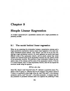
Confidence Intervals Obviously this model is subject to uncertainty, as the observed points do not normally all lie on a perfect straight line and are assumed to be a sample from a larger population. Thus the coefficients for the intercept and slope are only estimates of the true value. Confidence intervals can be calculated for these values to give a range of possible values. The 95% confidence intervals for the example in the Simple Linear Regression worksheet have been plotted on the graph below: The bold line is the original model The thin solid lines are models using the upper and lower bounds for the constant The short dashed lines are models using the lower bound for the slope and the upper and lower bounds for the constant
Based on material provided by Loughborough University Mathematics Learning Support Centre and Coventry University Mathematics Support Centre
Simple Linear Regression The long dashed lines are models using the upper bound for the slope and the upper and lower bounds for the constant
Page 2 of 3
Confidence interval model lines for the constant and slope
These models emphasise the importance of only using the model to predict values within the region of the data.
Validity of simple linear regression Simple linear regression is based on the following assumptions: 1. Both variables are continuous 2. The observations are random samples from normal distributions. However, according to Kleinbaum et al. (1998, p. 117), “normality is not necessary for the least-squares fitting of the regression model but it is required in general for inference making” (e.g. calculating the p-values and the confidence intervals of b0 and b1) “only extreme departures of the distribution of y from normality yield spurious results”. 3. The data values are independent of each other, i.e. only one pair of readings per participant is used 4. There is a linear relationship between the two variables and a good theoretical rationale for assuming one variable depends on another in a linear way 5. The relationship between the two variables is homoscedastic (i.e. the variance of one variable is the same for all the values of the other variable). Assumptions 3, 4 and 5 can be evaluated simultaneously by looking for an approximate cigar shaped scatter plot (see Simple Linear Regression worksheet). 6. The residuals are normally distributed with constant variance. This can be tested in SPSS by looking at the standardised residuals against the standardised predicted values and a normal probability plot: o Select Analyze – Regression – Linear o Choose the dependent and independent variable as before o Select Plots… o Select *ZRESID for the Y variable (standardised residual)
Based on material provided by Loughborough University Mathematics Learning Support Centre and Coventry University Mathematics Support Centre
Simple Linear Regression
Page 3 of 3
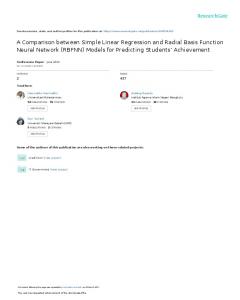
o Select *ZPRED for the X variable (standardised predicted value) o Select Normal probability plot The plotted points on the P-P plot should approximately fit the straight line. Any strong systematic curvature suggests some degree of nonnormality. This one is fine. The scatterplot of the standardised residuals against the predicted values should have a random pattern. Any discernible pattern (such as a ‘U’ shape) indicates a problem. This one is also fine.
Reference Kleinbaum, D., Kupper L., Muller K. and Nizam, A. (1998) Applied Regression Analysis and Multivariable Methods. 3rd ed. Pacific Grove, CA: Duxbury.